
TOF Spectrum (Time-of-Flight Histogram)
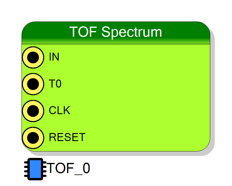
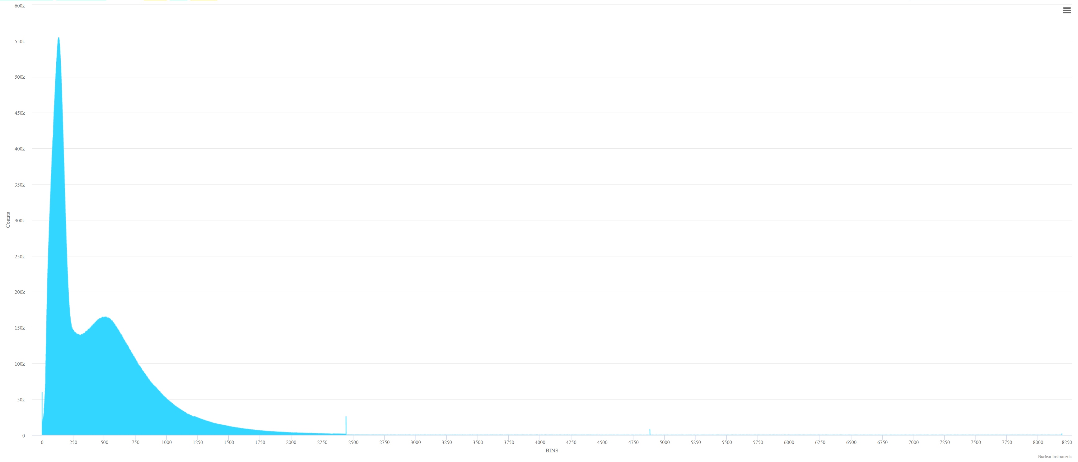
TOF_Spectrum builds a real-time histogram of time-of-flight measurements. It measures the time between a reference signal (T0) and detector events (IN), accumulating counts into configurable time bins. Ideal for neutron scattering, mass spectrometry, and any application requiring time-of-arrival distributions.
Introduction
Principle of Operation
The TOF Spectrum block implements a 1D histogram that accumulates time-of-flight measurements in real-time on the FPGA.
Unlike the standard Spectrum block (which histograms amplitude values), the TOF Spectrum measures time intervals between:
- T0: Reference timing signal (e.g., accelerator pulse, chopper, trigger)
- IN: Detector event signal
Each time bin corresponds to a specific time window after T0:
$$ bin_{index} = \left\lfloor \frac{t_{event} - t_{T0} - T_{delay}}{T_{bin}} \right\rfloor $$
where:
- $t_{event}$ = time of detector event (IN rising edge)
- $t_{T0}$ = time of reference signal (T0 rising edge)
- $T_{delay}$ = configurable start delay
- $T_{bin}$ = configurable bin width (in clock cycles)
Pin Description
Properties
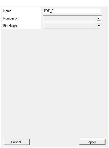
Set the name of the endpoint
Logical endpoint name used in the register map. Used by Resource Explorer and SciSDK.Default: TOF_0
Number of bins in the spectrum
Number of time bins in the histogram. Options: 32, 64, 128, 256, 512, 1024, 2048, 4096, 8192, 16384. More bins = longer measurement window or finer resolution.Default: 1024
Options: 32 64 128 256 512 1024 2048 4096 8192 16384
Height in bits of each bin
Number of bits per bin (maximum counts per bin). Options: 16, 24, 32 bits.
| Bits | Max Counts |
|---|---|
| 16 | 65,535 |
| 24 | 16,777,215 |
| 32 | 4,294,967,295 |
Default: 24
Options: 16 24 32
Detailed Operation
Data Flow
┌─────────────────────────────────────────────────────────────────────┐
│ TOF Spectrum Data Flow │
│ │
│ T0 ────────►┌──────────────┐ │
│ │ Time │ ┌─────────────┐ │
│ IN ────────►│ Counter │────►│ Memory │───► PC │
│ │ + Hist │ │ (N bins) │ │
│ CLK ───────►│ │ │ │ │
│ └──────────────┘ └─────────────┘ │
│ │ │
│ ┌────┴────┐ │
│ │ STATUS │──► Running/Idle/Completed │
│ └─────────┘ │
└─────────────────────────────────────────────────────────────────────┘
Operation Sequence
- Software configures bin width and start delay via registers
- Software starts acquisition via CONFIG register
- On T0 rising edge:
- Time counter resets to zero
- After start delay, histogram accumulation begins
- On each IN rising edge:
- Current time bin is incremented
- Events are accumulated until bin window ends
- Time counter advances through all bins
- Process repeats on next T0
Timing Diagram
State Machine
The block implements a 7-state FSM:
| State | Code | Description |
|---|---|---|
| CLEAR_START | 000 | Begin memory clear |
| CLEARING | 001 | Clear all bins to zero |
| RESET_DONE | 111 | Ready for acquisition |
| WAIT_DELAY | 010 | Wait for start delay after T0 |
| HISTOGRAM | 011 | Active histogramming |
| SAVE_RAM | 100 | Write accumulated count to RAM |
| SAVE_RAM_2 | 101 | RAM write completion |
| SCAN_DONE | 110 | Acquisition complete |
Configuration Parameters
| Parameter | Register | Description |
|---|---|---|
| Bin Width | CONFIG_BINWIDTH | Width of each time bin in clock cycles |
| Start Delay | CONFIG_START_DELAY | Delay from T0 before starting histogram |
| Start/Stop | CONFIG[0] | 1 = Start, 0 = Stop |
| Reset | CONFIG[1] | 1 = Clear histogram |
Time Resolution
The time resolution depends on the clock frequency and bin width:
$$ \Delta t = \frac{T_{bin}}{f_{CLK}} $$
| Clock | Bin Width | Time Resolution |
|---|---|---|
| 125 MHz | 1 | 8 ns |
| 125 MHz | 10 | 80 ns |
| 125 MHz | 100 | 800 ns |
| 500 MHz | 1 | 2 ns |
| 500 MHz | 10 | 20 ns |
Total Measurement Window
$$ T_{window} = N_{bins} \times T_{bin} / f_{CLK} $$
| Bins | Bin Width | Clock | Window |
|---|---|---|---|
| 1024 | 100 | 125 MHz | 819.2 µs |
| 4096 | 10 | 125 MHz | 327.7 µs |
| 8192 | 1 | 500 MHz | 16.4 µs |
Use Cases
- Neutron scattering: Time-of-flight from chopper to detector
- Mass spectrometry: Ion flight time distribution
- Particle physics: Time-of-arrival histograms
- LIDAR: Round-trip time distribution
- Fluorescence lifetime: Decay time histograms
Software Integration
The TOF Spectrum is memory-mapped and can be read via SciSDK.
Available SDK Functions
| Function | Description |
|---|---|
SPECTRUM_<name>_START |
Start acquisition |
SPECTRUM_<name>_STOP |
Stop acquisition |
SPECTRUM_<name>_RESET |
Clear histogram |
SPECTRUM_<name>_SET_PARAMETERS |
Configure bin width and start delay |
SPECTRUM_<name>_STATUS |
Get acquisition status |
SPECTRUM_<name>_DOWNLOAD |
Read histogram data |
Status Values
| Value | Meaning |
|---|---|
| 0 | Stopped |
| 1 | Running |
| 2 | Idle (completed) |
| 4 | Clearing |
Python Example
python
from scisdk.scisdk import SciSDK
sdk = SciSDK()
sdk.AddNewDevice("usb:10500", "dt5560", "board0", "RegisterFile.json")
# Configure: 100 clock cycles per bin, 10 cycles start delay
sdk.SetParameter("board0:/MMCComponents/TOF_0.bin_width", 100)
sdk.SetParameter("board0:/MMCComponents/TOF_0.start_delay", 10)
# Reset and start
sdk.ExecuteCommand("board0:/MMCComponents/TOF_0.reset", "")
sdk.ExecuteCommand("board0:/MMCComponents/TOF_0.start", "")
# Wait for data...
time.sleep(10)
# Read histogram
res, data = sdk.ReadData("board0:/MMCComponents/TOF_0")
# Plot TOF spectrum
import matplotlib.pyplot as plt
plt.bar(range(len(data)), data)
plt.xlabel("Time Bin")
plt.ylabel("Counts")
plt.title("Time-of-Flight Spectrum")
plt.show()
Resources & Timing
-
Latency: 2-3 clock cycles from IN edge to bin update
-
Throughput: Multiple events per bin can be accumulated
- Uses dual-port BRAM for histogram storage
- One port for time-domain accumulation
- Second port for software readout
- Bin saturation prevents overflow wrap-around
- T0 resets time counter for each measurement cycle