
Pole-Zero TM
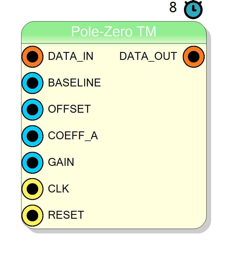
Time-multiplexed digital Pole-Zero Compensation (deconvolution) filter with programmable decay constant and gain. Removes the exponential tail from preamplifier signals, enabling higher count rates and improved pile-up rejection.
Introduction
The Pole-Zero TM block implements digital pole-zero cancellation (deconvolution) on time-multiplexed input signals. This is essential for processing signals from charge-sensitive preamplifiers, which produce exponentially decaying pulses.
The core uses Xilinx HLS (High-Level Synthesis) for efficient FPGA implementation, achieving a throughput of 1 word per clock cycle (II=1) while processing multiple TM samples in parallel.
By removing the exponential tail, the pole-zero compensation:
- Reduces pile-up at high count rates
- Improves baseline restoration
- Enables faster shaping times
Pin Description
a in 32-bit fixed-point format.
Format: 2 integer bits, 30 fractional bits (Q2.30).
Calculated as: COEFF_A = int(exp(-Ts/tau) * 2^30)
where Ts is sampling period and tau is preamplifier decay time.
GAIN = int((1/(1-a)) * 2^16)
Typical values: 1000-10000 depending on tau/Ts ratio.
Properties
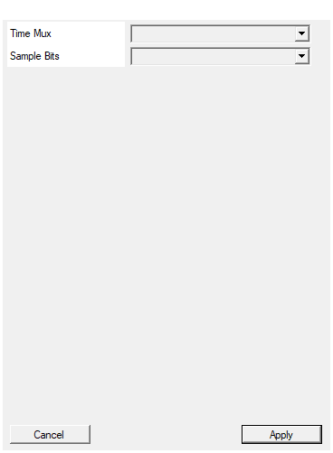
Set number of samples for each clock cycle
Number of parallel samples processed per clock cycle (TM factor). Available values: 2, 4, 8, 16, 32, default 4.Default: 4
Options: 2 4 8 16 32
Set number of bits for each sample
Bit-width of each sample within the TM frame. Applies toDATA_IN, BASELINE, OFFSET and DATA_OUT signals.
Available values: 8, 10, 12, 14, 16, 18, 20, 22, 24, default 16.
Default: 16
Options: 8 10 12 14 16 18 20 22 24
Usage
Signal Processing Overview
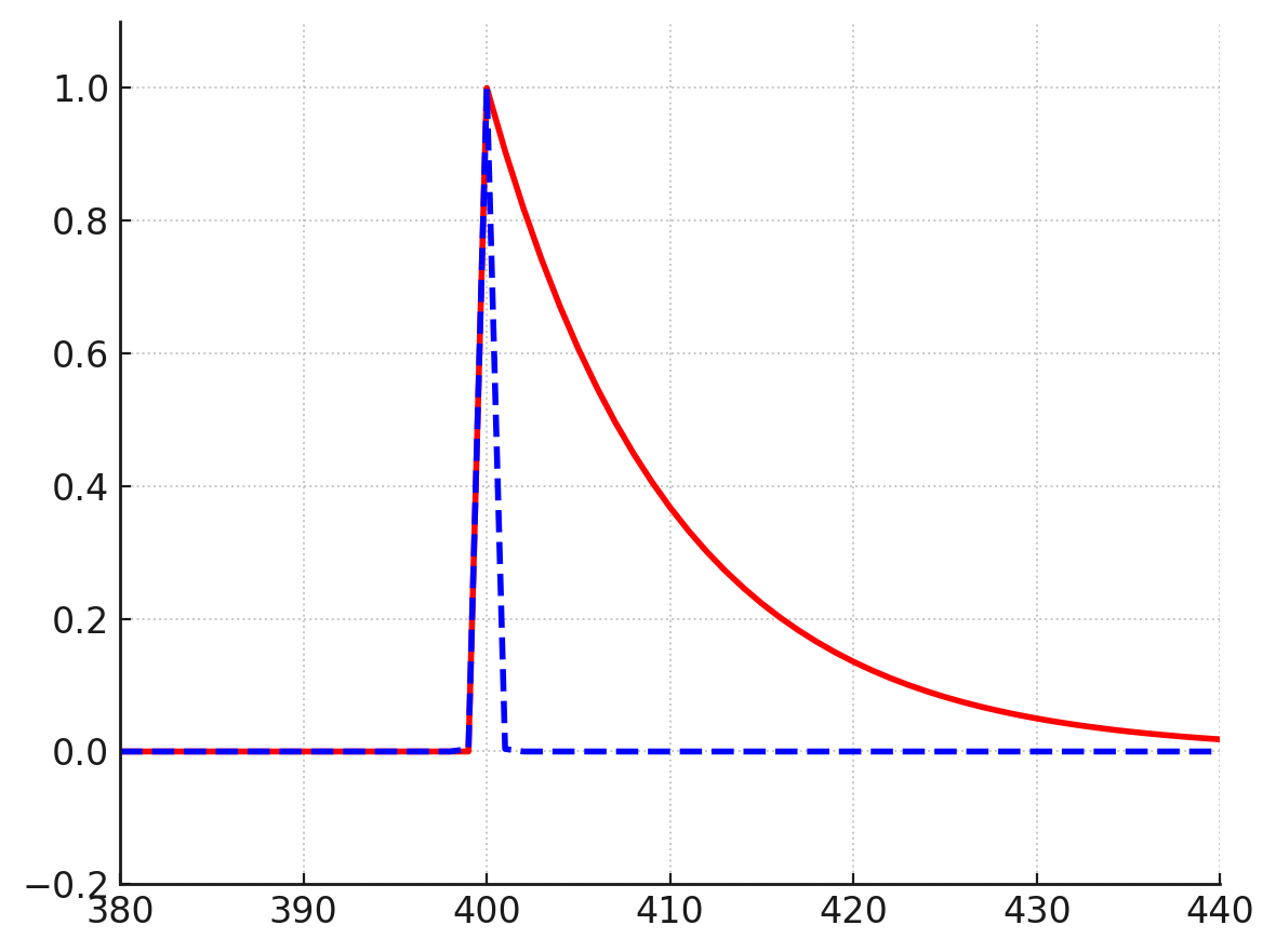
The figure shows the effect of pole-zero compensation on an exponentially decaying signal. The original signal (with long exponential tail) is transformed into a much shorter pulse, allowing the system to process events more closely spaced in time.
Transfer Function
The pole-zero compensation implements a first-order digital high-pass filter with the transfer function:
$$ H(z) = \text{gain} \cdot (1 - a \cdot z^{-1}) $$
In the time domain, for each sample:
$$ y[n] = \text{gain} \cdot (x[n] - a \cdot x[n-1]) $$
where:
x[n]is the baseline-subtracted input sampley[n]is the output sampleais the pole-zero coefficient (COEFF_A)gaincompensates for the amplitude reduction
Calculating COEFF_A from Decay Time Constant
The pole-zero coefficient a must be matched to the preamplifier decay time constant τ:
$$ a = e^{-T_s / \tau} $$
where:
- $T_s$ is the sampling period (1 / sampling_frequency)
- $\tau$ is the preamplifier decay time constant
Fixed-point representation:
The coefficient is represented as a 32-bit fixed-point number with 2 integer bits and 30 fractional bits:
$$ \text{COEFF_A} = \left\lfloor a \cdot 2^{30} \right\rfloor $$
Example calculation (Python):
python
import math
sampling_freq = 125e6 # 125 MHz
tau = 50e-6 # 50 µs preamplifier decay time
Ts = 1.0 / sampling_freq # 8 ns
a = math.exp(-Ts / tau) # ≈ 0.99984
COEFF_A = int(a * (2**30))
# Result: COEFF_A = 1073569465 (0x3FFD4339)
Calculating GAIN
To compensate for the amplitude reduction caused by the differentiation, a gain factor is applied:
$$ \text{gain} = \frac{1}{1 - a} \approx \frac{\tau}{T_s} $$
Fixed-point representation:
The gain is represented as a 32-bit fixed-point number with 16 integer bits and 16 fractional bits:
$$ \text{GAIN} = \left\lfloor \text{gain} \cdot 2^{16} \right\rfloor $$
Example calculation (Python):
python
gain = 1.0 / (1.0 - a) # ≈ 6250 for the above example
GAIN = int(gain * (2**16))
# Result: GAIN = 409600000 (0x186A0000)
Baseline Subtraction
The block subtracts a programmable BASELINE value from each input sample before processing. This allows:
- Removal of DC offset from the ADC
- Compensation for baseline drift
- Centering the signal around zero for proper deconvolution
Output Offset
After deconvolution, the OFFSET value is added to shift the output signal to the desired range. This is useful when:
- The downstream processing expects unsigned values
- A specific DC level is required for triggering
Time-Multiplexed Processing
The block processes TM samples per clock cycle in parallel. The state variable x_prev (last sample of the previous word) is maintained across clock cycles to ensure continuity of the filtering operation.
Fixed-Point Precision
Internal calculations use extended precision to prevent overflow:
- coeff_t: 32 bits, 2 integer bits, 30 fractional bits (for coefficient a)
- gain_t: 32 bits, 16 integer bits, 16 fractional bits (for gain)
- signal_t: 32 bits, 17 integer bits, 15 fractional bits (for signals)
- accum_t: 48 bits, 33 integer bits, 15 fractional bits (for accumulator)
Latency
- Processing latency: 8 clock cycles from input to output
- Throughput: TM samples per clock cycle (fully pipelined, II=1)
Typical Applications
- Signal conditioning for charge-sensitive preamplifiers
- Pile-up reduction in high count-rate spectroscopy
- Pre-processing for trapezoidal shapers
- Baseline restoration in MCA systems