
Random Generator (Arbitrary Distribution)
Generates random numbers that follow an ARBITRARY distribution, not just a uniform or a Gaussian one. The distribution is drawn in the Distribution Designer – from 58 built-in measured spectra, 20 analytic shapes, or an imported file – and baked into a lookup table at compile time.
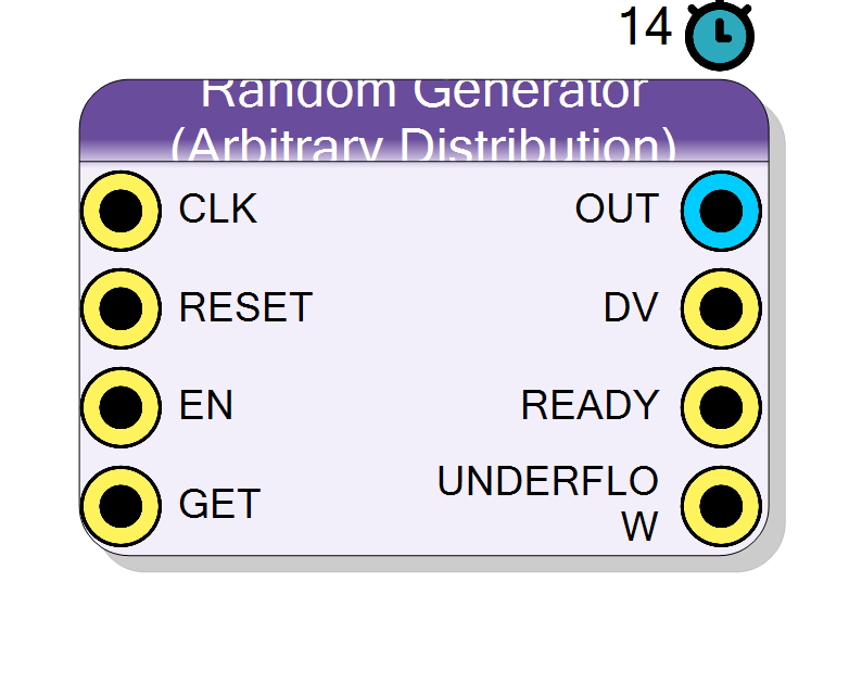
Introduction
The Random Generator (Arbitrary Distribution) block produces a stream of random values whose histogram reproduces any distribution you give it.
It implements inverse transform sampling (also called the inversion method or the Smirnov transform), the standard way to sample an arbitrary distribution:
1. tabulate the CUMULATIVE histogram (CDF) of the wanted distribution
2. draw a uniform random number u
3. find the bin where u falls on the CDF
4. that bin index IS the random value
Because the CDF is monotonic, step 3 is a binary search, which is what makes the block cheap: one table, one comparator, no multiplier, no divider and no DSP.
Double-click the block to open the Distribution Designer, where the distribution is chosen and the table is built.
Pin Description
Properties
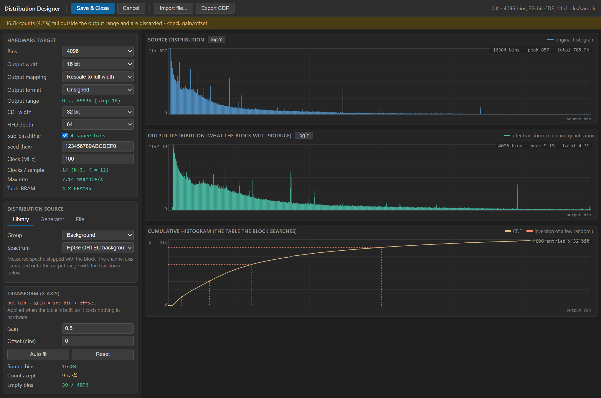
Configuration produced by the Distribution Designer. Double-click the block to edit it.
The whole configuration produced by the Distribution Designer: the hardware settings, the chosen source, the transform and the quantised cumulative table. Double-click the block to edit it; this field is not meant to be typed by hand.Number of CDF entries (set in the designer).
Number of entries in the cumulative table, 256 to 16384 (powers of two), default 4096. It sets both the resolution of the distribution and the sampling rate: one sample costslog2(Bins) + 2 clocks.
Set in the designer.
Default: 4096
Width of the OUT port (set in the designer).
Width of theOUT port, log2(Bins) to 32, default 16. The bin
index sits in the upper bits and the remaining low bits carry the
sub-bin dither. Set in the designer.
Default: 16
Depth of the output FWFT queue (set in the designer).
Depth of the output queue, 16 to 4096 (powers of two), default 64. Deeper absorbs longer read bursts; the generator stalls while it is full. Set in the designer.Default: 64
Which distribution is loaded (set in the designer).
Read-only reminder of which distribution is loaded (library entry, analytic shape or imported file name).Range of the OUT port for the chosen mapping and format (set in the designer).
Read-only reminder of the rangeOUT will actually carry, for example
native 0..1023 or rescaled -32768..32767. Set in the designer through
Output mapping and Output format.
Default: rescaled 0..65535
Usage
Where the distribution comes from
The designer offers three sources, all ending in the same quantised table:
- Library – 58 real measured spectra shipped with the block: isotopes (Cs-137, Co-60, Am-241, Eu-152, Ba-133, K-40, Ra-226 …), samples and materials (KCl, Fiestaware, pitchblende, volcanic material, Chernobyl grass …), HpGe backgrounds and a He-3 neutron spectrum.
- Generator – 20 analytic shapes: Gaussian, uniform, exponential, log-normal, gamma, beta, Weibull, Rayleigh, Maxwell-Boltzmann, chi-squared, Student’s t, Cauchy/Lorentzian, Laplace, triangular, Landau (Moyal approximation, for energy loss), Poisson, binomial, geometric, plus a detector spectrum builder (any number of Gaussian peaks over an exponential Compton-like continuum and a flat background).
- File – CSV / TXT (one count per line, or
x,ypairs) and JSON (a flat array of counts).
Shaping the distribution
The designer maps the source onto the output range with
out_bin = gain x src_bin + offset
applied when the table is built, so it costs nothing in hardware. The three plots show the original histogram, the histogram the block will actually produce (after rebinning and quantisation) and the cumulative histogram with the graphical inversion. Auto fit picks gain and offset that map the non-empty part of the source onto the whole output range.
Rebinning conserves COUNTS, not sample values: a source bin is spread over the output bins it overlaps in proportion to the overlap, so the areas – that is, the probabilities – are preserved.
Output value
Two independent choices decide what number comes out of OUT.
Output mapping – how the bin index becomes a value:
- Bin index –
OUTis the bin number itself,0 .. Bins-1. With 1024 bins on a 16-bit port you get values0..1023, not0..65535. The port is simply wider than the numbers it carries. - Rescale to full width – the index is stretched over the whole output
width:
OUT = index x 2^(OutputWidth - log2(Bins)) + dither. With 1024 bins on a 16-bit port you get0..65535in steps of 64, and the 6 spare low bits are filled by the dither.
Output format – how that span is interpreted:
- Unsigned –
0 .. Bins-1(bin index) or0 .. 2^OutputWidth-1(rescaled). - Signed – the same span shifted to sit on zero, two’s complement:
-Bins/2 .. Bins/2-1(bin index) or-2^(OutputWidth-1) .. 2^(OutputWidth-1)-1(rescaled).
So 1024 bins on a 16-bit port can give you 0..1023, -512..511,
0..65535 or -32768..32767. The designer shows the resulting range live.
Sub-bin dithering only exists in rescale mode, because only there are
there bits below the index. It is not cosmetic: a histogram asserts a
constant density INSIDE a bin, so filling the sub-bin uniformly reproduces
exactly the tabulated distribution. With dithering off the rescaled output
is a comb of Bins codes with gaps between them. In bin index mode the
setting is ignored.
Rate, and why there is a FIFO
The binary search takes one clock per step, so one sample costs
log2(Bins) + 2 clocks
(14 clocks for 4096 bins). That is the block’s natural rate – for example ~7.1 Msample/s at 100 MHz with 4096 bins. The output queue decouples that fixed rate from whatever consumes the samples.
Reading a sample: request, then strobe
clock N GET pulses high for one clock
clock N+1 OUT carries the new sample and DV is high, for exactly
one clock
DVis a strobe, not a level: it marks the clock on which a freshly delivered sample appears. Between strobesOUTsimply holds the last sample delivered.READYtells you whether aGETwill succeed: it is high while at least one sample is queued. GateGETwith it, or accept the underflow.UNDERFLOWpulses whenGETarrives on an empty queue. It comes from the Xilinx FIFO primitive and is registered, so it appears one clock after the offendingGET– in the cycleDVwould have occupied had the read succeeded. On such aGET,DVdoes not strobe.- When the queue is full the generator stops and restarts by itself as soon as a slot frees up. No sample is ever generated and thrown away.
Typical applications
- Detector emulation: feed a real measured spectrum into an MCA or DPP chain without a source and without a detector.
- Monte Carlo stimulus for trigger and pile-up algorithms.
- Realistic event-rate and amplitude generation for firmware self-test.
- Any application needing noise with a prescribed, non-Gaussian shape.
Reset
RESET clears the queue and reloads the RNG seed, so the sequence restarts
identically. Two blocks with the same seed produce the same stream: give
them different seeds when you need independent channels.
Resources & Timing
-
Latency: log2(Bins) + 2 clock cycles per sample (14 with the default 4096 bins)
-
Throughput: one sample every log2(Bins) + 2 clocks; the FIFO decouples the reader
No DSP and no multiplier: one comparator, one adder and the table. The table costs ceil(CdfWidth/36) x ceil(Bins/1024) BRAM36 (the designer shows the live figure) plus the output FIFO. Pure VHDL, no HLS. The random source is a 64-bit xorshift generator (period 2^64-1) and the output queue is a Xilinx XPM FIFO in standard read mode (one clock of read latency), which is what gives the GET-then-strobe protocol.