
Trapezoidal Shaper FP
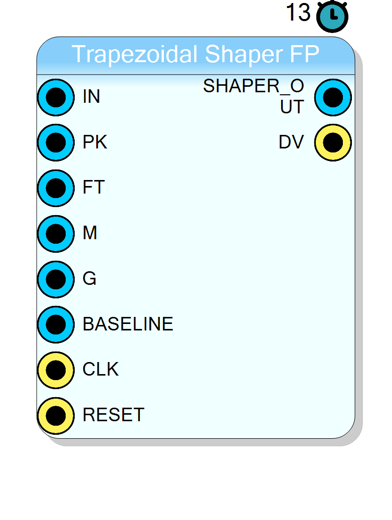
Floating-point trapezoidal shaper with integrated pole-zero compensation (deconvolution). Transforms exponentially decaying preamplifier pulses into trapezoidal waveforms for optimal pulse-height analysis.
Introduction
The Trapezoidal Shaper FP block implements a recursive digital trapezoidal filter based on the Jordanov-Knoll algorithm (1994). This filter transforms exponentially decaying signals from charge-sensitive preamplifiers into trapezoidal waveforms, which are optimal for pulse-height analysis.
The block includes integrated pole-zero compensation (deconvolution) using the M coefficient, eliminating the need for a separate deconvolution stage.
This is a floating-point implementation that provides high accuracy for the deconvolution coefficient M and the gain G.
Pin Description
M = 1 / (exp(Ts/tau) - 1)
where Ts is sampling period and tau is preamplifier decay time.
IEEE 754 single-precision format.
Properties
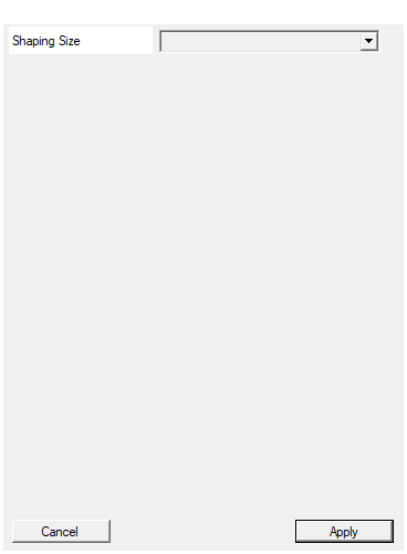
Set the maximum number of samples supported by the MCA. This will affect the trapezoidal shaper and the baseline restorer
Maximum number of samples supported by the delay lines. Determines the maximum values for PK and FT parameters. Must be larger thanmax(PK, PK+FT).
Available values: 1024, default 1024.
Default: 1024
Options: 1024
Usage
Filter Structure
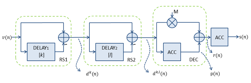
The figure shows the recursive structure of the trapezoidal filter:
- RS1: First running sum stage with delay k (peaking time)
- RS2: Second running sum stage with delay l (flat-top time)
- DEC: Deconvolution stage with coefficient M and accumulator
- ACC: Final accumulator for output generation
Algorithm Overview
The trapezoidal shaper processes the input signal through four stages:
Stage 1 - First Difference (d^k)
$$ d^k[n] = v[n] - v[n-k] $$
This implements a moving-average filter (boxcar) with window size k. The parameter k is the peaking time in clock cycles.
Stage 2 - Second Difference (d^{k,l})
$$ d^{k,l}[n] = d^k[n] - d^k[n-l] $$
This creates the flat-top portion of the trapezoid. The parameter l = k + FT, where FT is the flat-top duration in clock cycles.
Stage 3 - Deconvolution with M coefficient
$$ p[n] = p[n-1] + d^{k,l}[n] $$ $$ r[n] = p[n] + M \cdot d^{k,l}[n] $$
The M coefficient performs pole-zero cancellation of the preamplifier decay.
Stage 4 - Final Accumulation with Gain
$$ s[n] = s[n-1] + G \cdot r[n] $$
The gain G compensates for the amplitude reduction and provides output scaling.
Calculating the M Coefficient
The deconvolution coefficient M must be matched to the preamplifier decay time constant τ:
$$ M = \frac{1}{e^{T_s / \tau} - 1} $$
where:
- $T_s$ is the sampling period (1 / clock_frequency)
- $\tau$ is the preamplifier decay time constant
Example calculation (Python):
python
import math
clock_freq = 125e6 # 125 MHz
tau = 50e-6 # 50 µs preamplifier decay time
Ts = 1.0 / clock_freq # 8 ns
M = 1.0 / (math.exp(Ts / tau) - 1)
# Result: M ≈ 6249.0
For typical systems:
- f_clock = 65 MHz, τ = 2 µs: M ≈ 33
- f_clock = 125 MHz, τ = 50 µs: M ≈ 6249
- f_clock = 250 MHz, τ = 100 µs: M ≈ 24999
Calculating the Gain G
The gain G is typically set to normalize the output amplitude:
$$ G = \frac{\text{desired_output_scale}}{k} $$
A common starting value is G = 1.0, then adjusted empirically for optimal dynamic range.
Trapezoidal Shape Parameters
The output waveform shape is determined by:
- Rise time: k clock cycles (set by PK input)
- Flat-top duration: FT clock cycles (set by FT input)
- Fall time: k clock cycles (symmetric with rise time)
Total shaping time = 2k + FT clock cycles
Advantages of Trapezoidal Shaping
- Noise Reduction: Optimal signal-to-noise ratio for both series and parallel noise components
- Ballistic Deficit Control: Adjustable flat-top compensates for charge collection time variations
- High Count Rate: Faster shaping times compared to Gaussian shapers
- Pile-up Rejection: Well-defined pulse boundaries simplify pile-up detection
Timing and Latency
- Processing latency: 13 clock cycles from input to output
- Throughput: 1 sample per clock cycle (fully pipelined)
Typical Applications
- Gamma-ray spectroscopy with HPGe detectors
- X-ray spectroscopy with SDD detectors
- Multi-Channel Analyzer (MCA) front-end
- Nuclear physics pulse processing