
FFT Monitor
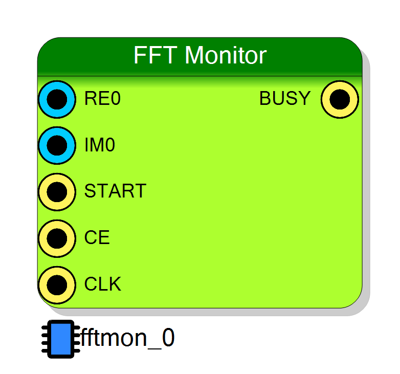
Transfers FFT real and imaginary data to the PC for magnitude and phase spectrum visualization. Works in conjunction with the Math→FFT block for real-time spectrum analysis. Supports up to 8 simultaneous channels with configurable FFT size from 128 to 16384 bins.
Introduction
Principle of Operation
The FFT Monitor block transfers the real and imaginary parts of FFT data to the PC, enabling real-time calculation and display of magnitude and phase spectra.
Let:
- $X[k] = RE[k] + j \cdot IM[k]$ = complex FFT output at bin $k$
- $N$ = number of FFT bins (samples per channel)
- $f_s$ = sampling frequency of the original time-domain signal
The frequency resolution is: $$ \Delta f = \frac{f_s}{N} $$
And the frequency of bin $k$ is: $$ f_k = k \cdot \Delta f = \frac{k \cdot f_s}{N} $$
This block is designed to work in conjunction with the Math → FFT block. Connect the FFT output (RE, IM) to this monitor to visualize the frequency spectrum using Resource Explorer or read data programmatically with SciSDK.
SciSDK Documentation: https://nuclearinstruments.github.io/SCISDK/
Pin Description
Properties
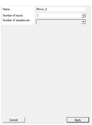
Set the name of the endpoint
Logical endpoint name used in register map. Used to identify the component in Resource Explorer and SciSDK. Default: fftmon_0Default: fftmon_0
Set the number of input to the virtual block
Number of FFT channels to monitor (1-8). Each channel has its own RE and IM inputs. Default: 1Default: 1
Range: 1 – 8
Set the number of samples stored for each acquisition
Number of FFT bins to capture per channel. Should match the FFT size. Available values: 128, 256, 512, 1024, 2048, 4096, 8192, 16384. Default: 4096Default: 4096
Options: 128 256 512 1024 2048 4096 8192 16384
⚙️ Detailed Operation
Data Flow
- Connect the RE (real) and IM (imaginary) outputs from an FFT block
- The START signal triggers data capture (should align with first FFT output sample)
- While CE is HIGH, samples are captured on each clock cycle
- Data is transferred to the PC for magnitude/phase calculation
┌──────────────────────────────────────────────────────────────────┐
│ FFT Monitor Data Flow │
│ │
│ ┌─────────┐ ┌─────────────┐ │
│ │ │──RE──►┌──────────┐ │ │ │
│ │ FFT │ │ FFT │ │ Mag/Phase │ │
│ │ Block │──IM──►│ Monitor │─┼─► Spectrum │ │
│ │ │ │ │ │ │ │
│ └─────────┘ └──────────┘ └─────────────┘ │
│ │ ▲ ▲ │
│ │ │ │ │
│ └──────START───────┘ Resource Explorer │
│ or SciSDK │
└──────────────────────────────────────────────────────────────────┘
Typical Usage
The FFT Monitor is typically connected to an FFT block to create a spectrum analyzer:
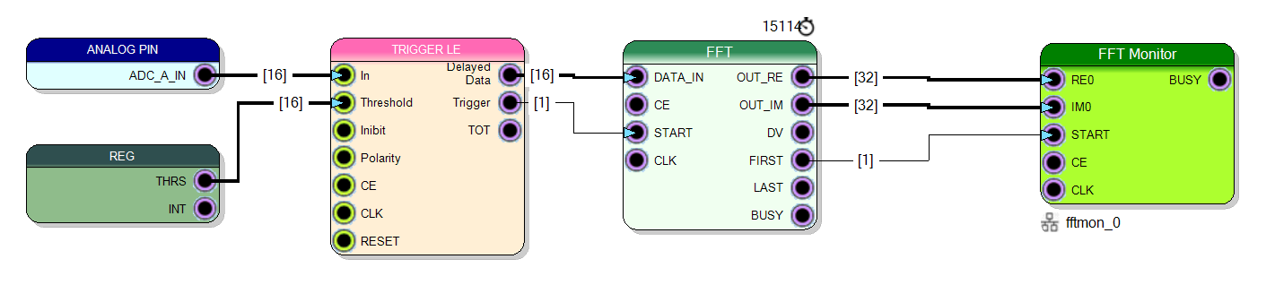
In this configuration:
- The FFT block computes the Fast Fourier Transform of the input signal
- The FFT Monitor captures the complex output (RE + jIM)
- Resource Explorer or SciSDK displays the magnitude and phase spectra
Magnitude and Phase Calculation
The PC-side software (or SciSDK in decoded mode) calculates:
Magnitude (Power Spectrum): $$ |X[k]| = \sqrt{RE[k]^2 + IM[k]^2} $$
Phase: $$ \phi[k] = \text{atan2}(IM[k], RE[k]) $$
Power Spectral Density (optional normalization): $$ PSD[k] = \frac{|X[k]|^2}{N} $$
Magnitude in dB: $$ |X[k]|{dB} = 20 \cdot \log{10}(|X[k]|) $$
Multi-Channel Support
The FFT Monitor supports up to 8 channels, allowing simultaneous monitoring of multiple FFT outputs. Each channel has its own RE and IM inputs (RE0/IM0, RE1/IM1, …, RE7/IM7).
Memory Organization
FFT data is stored in BRAM with the following layout:
| Address Range | Content |
|---|---|
| 0 to N-1 | Channel 0: RE[0..N-1] |
| N to 2N-1 | Channel 0: IM[0..N-1] |
| 2N to 3N-1 | Channel 1: RE[0..N-1] |
| … | … |
Total memory per channel: $2N$ words (32-bit each for RE and IM).
Software Integration with SciSDK
The FFT Monitor is fully supported by SciSDK. For complete documentation see: SciSDK FFT Guide
Data Processing Modes
| Mode | Description | Use Case |
|---|---|---|
| raw | Returns raw RE/IM data as 32-bit integers | High-speed logging, custom processing |
| decoded | Pre-calculated magnitude and phase as double | Real-time display, easy integration |
Available Parameters
| Parameter | Access | Description | Default |
|---|---|---|---|
decimator |
R/W | X-axis decimation factor $D$, skips $2^D$ bins | 0 |
auto_arm |
R/W | Enable automatic trigger arming | 1 |
data_processing |
R/W | raw or decoded mode |
decoded |
acq_mode |
R/W | blocking or non-blocking |
blocking |
timeout |
R/W | Timeout in milliseconds for blocking mode | 5000 |
Available Commands
| Command | Description |
|---|---|
arm |
Manually trigger acquisition (when auto_arm = 0) |
reset_read_valid_flag |
Reset data ready flag |
Raw Data Decoding (Software)
When using raw mode, decode as follows:
c
// Raw buffer contains interleaved RE/IM for each channel
int32_t re = raw_data[2*k]; // Real part of bin k
int32_t im = raw_data[2*k + 1]; // Imaginary part of bin k
// Calculate magnitude and phase
double magnitude = sqrt((double)re*re + (double)im*im);
double phase = atan2((double)im, (double)re);
C/C++ Example
c
#include "SciSDK_DLL.h"
#include <math.h>
// Allocate decoded buffer
SCISDK_FFT_DECODED_BUFFER *buffer;
SCISDK_AllocateBuffer("board0:/MMCComponents/fftmon_0",
T_BUFFER_TYPE_DECODED,
(void**)&buffer, _sdk);
// Configure
SCISDK_SetParameterString("board0:/MMCComponents/fftmon_0.data_processing",
"decoded", _sdk);
SCISDK_SetParameterString("board0:/MMCComponents/fftmon_0.acq_mode",
"blocking", _sdk);
// Read spectrum data
int ret = SCISDK_ReadData("board0:/MMCComponents/fftmon_0",
(void*)buffer, _sdk);
if (ret == NI_OK) {
int N = buffer->info.samples;
// Find peak frequency
double max_mag = 0;
int peak_bin = 0;
for (int k = 0; k < N/2; k++) { // Only positive frequencies
if (buffer->mag[k] > max_mag) {
max_mag = buffer->mag[k];
peak_bin = k;
}
}
// Calculate peak frequency (assuming fs = 100 MHz)
double fs = 100e6;
double peak_freq = (double)peak_bin * fs / N;
printf("Peak at bin %d, frequency %.2f MHz, magnitude %.2f\n",
peak_bin, peak_freq/1e6, max_mag);
}
// Free buffer
SCISDK_FreeBuffer("board0:/MMCComponents/fftmon_0",
T_BUFFER_TYPE_DECODED, (void**)&buffer, _sdk);
Python Example
python
from scisdk.scisdk import SciSDK
import numpy as np
import matplotlib.pyplot as plt
sdk = SciSDK()
sdk.AddNewDevice("usb:10500", "dt5560", "board0", "RegisterFile.json")
# Allocate buffer
res, buf = sdk.AllocateBuffer("board0:/MMCComponents/fftmon_0",
sdk.T_BUFFER_TYPE_DECODED)
# Configure
sdk.SetParameter("board0:/MMCComponents/fftmon_0.data_processing", "decoded")
sdk.SetParameter("board0:/MMCComponents/fftmon_0.acq_mode", "blocking")
# Read spectrum
res, buf = sdk.ReadData("board0:/MMCComponents/fftmon_0", buf)
if res == 0:
N = len(buf.mag)
fs = 100e6 # Sampling frequency
# Create frequency axis
freq = np.arange(N) * fs / N
# Plot magnitude spectrum (only positive frequencies)
plt.figure(figsize=(12, 8))
plt.subplot(2, 1, 1)
plt.plot(freq[:N//2] / 1e6, 20*np.log10(buf.mag[:N//2] + 1e-10))
plt.title("Magnitude Spectrum")
plt.xlabel("Frequency (MHz)")
plt.ylabel("Magnitude (dB)")
plt.grid(True)
# Plot phase spectrum
plt.subplot(2, 1, 2)
plt.plot(freq[:N//2] / 1e6, np.rad2deg(buf.ph[:N//2]))
plt.title("Phase Spectrum")
plt.xlabel("Frequency (MHz)")
plt.ylabel("Phase (degrees)")
plt.grid(True)
plt.tight_layout()
plt.show()
Resource Explorer
Resource Explorer can connect directly to the FFT Monitor endpoint to display real-time magnitude and phase spectra without writing any code.
Quick Reference
| Item | Formula / Meaning |
|---|---|
| Frequency resolution | $\Delta f = f_s / N$ |
| Bin frequency | $f_k = k \cdot f_s / N$ |
| Magnitude | $|X[k]| = \sqrt{RE^2 + IM^2}$ |
| Phase | $\phi = \text{atan2}(IM, RE)$ |
| Nyquist bin | $k_{Nyquist} = N/2$ |
| Max detectable frequency | $f_{max} = f_s / 2$ |
Resources & Timing
-
Latency: Capture starts on START pulse, ~2 clock cycles pipeline
-
Throughput: One complex sample (RE+IM) per clock cycle
- Uses BRAM for sample storage (2N words per channel)
- Supports up to 8 simultaneous channels
- Resource Explorer provides real-time spectrum display
- SciSDK supports both raw and decoded readout modes
- Decoded mode provides pre-calculated magnitude and phase