
FLOATING POINT - NATURAL LOGARITHM
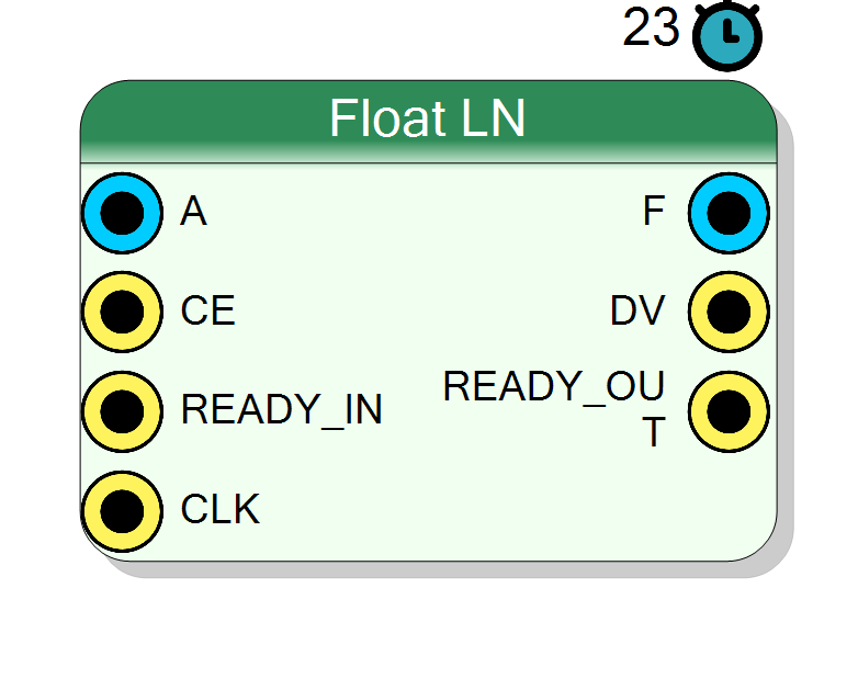
Computes the natural logarithm (ln) of IEEE-754 floating-point numbers with configurable DSP usage. Supports both single-precision (32-bit) and double-precision (64-bit) formats. Built on Xilinx Floating-Point IP core with blocking flow control and 23-cycle latency.
Introduction
The block computes the natural logarithm of IEEE-754 floating-point inputs.
On every rising edge of CLK, if CE = 1, the logarithm unit computes
$$ \mathrm{F}(n) = \ln(\mathrm{A}(n)), $$
where input A and output F follow IEEE-754 single or double
precision format.
The logarithm is implemented with the Xilinx floating_point IP core configured for Logarithm operation using polynomial approximation with blocking flow control, fixed 23-cycle latency, and configurable DSP primitive usage.
Pin Description
CE = 1 and READY_OUT = 1.
CE = 1, input A is accepted and logarithm computation begins. Can be tied to ‘1’ for continuous operation.
DV = 1.
Result = ln(A).
F contains a valid logarithm.
Asserts 23 clock cycles after corresponding CE = 1.
Properties
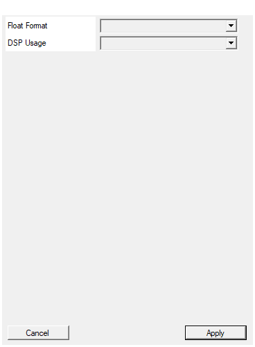
Select between single precision 32 bit and double precision 64 bit
Floating-point precision for both input and output:
- Single → 32-bit (8-bit exponent, 24-bit mantissa including implicit bit)
- Double → 64-bit (11-bit exponent, 53-bit mantissa including implicit bit)
The operation preserves the precision format end-to-end.
Default: Single
Options: Single Double
DSP Usage. Single precision: No [0], Medium [4], Full[13]. Double precision: No[0], Medium [23], Full[61]
DSP primitive allocation for polynomial evaluation:
- No_Usage → LUT-only (0 DSPs, lower speed, higher LUT usage)
- Medium_Usage → Partial DSP (4/23 DSPs for Single/Double)
- Full_Usage → Full DSP optimization (13/61 DSPs, higher speed, lower LUT usage)
Medium usage provides a good balance between resources and performance. Full usage is recommended for high-speed applications.
Default: Medium_Usage
Options: No_Usage Medium_Usage Full_Usage
Functional description
The component computes the natural logarithm:
$$ F = \ln(A) = \log_e(A) $$
The implementation uses polynomial approximation over normalized mantissa ranges, combined with exponent-based range reduction:
$$ \ln(x) = \ln(m \times 2^e) = \ln(m) + e \cdot \ln(2) $$
where $m \in [1, 2)$ is the normalized mantissa and $e$ is the exponent.
Special cases
IEEE-754 special value handling:
ln(1) = 0ln(+0) = -Infln(x) = NaNforx < 0(domain error)ln(+Inf) = +Infln(NaN) = NaN(NaN propagation)
DSP Usage
The DSP Usage property controls polynomial evaluation resources:
Single precision:
- No_Usage → Pure LUT implementation (0 DSPs, lower speed)
- Medium_Usage → Partial DSP optimization (4 DSPs)
- Full_Usage → Full DSP optimization (13 DSPs, higher speed)
Double precision:
- No_Usage → Pure LUT implementation (0 DSPs, lower speed)
- Medium_Usage → Partial DSP optimization (23 DSPs)
- Full_Usage → Full DSP optimization (61 DSPs, higher speed)
Higher DSP usage improves timing and reduces LUT consumption at the cost of DSP48 primitives.
Timing
The IP has a fixed 23-cycle pipeline latency:
| Clock cycle | Event |
|---|---|
| 0 | Input A presented with CE = 1 |
| 23 | Output F valid with DV = 1 |
The READY_IN/READY_OUT handshake signals enable backpressure control for streaming applications.
Typical use cases
- Signal compression (logarithmic amplitude)
- Decibel conversion (20×log10 = 20×ln/ln(10))
- Information theory calculations (entropy, mutual information)
- Machine learning (log-likelihood computations)