
ALU - IIR AVERAGE
Configurable IIR (Infinite Impulse Response) averaging filter implemented via Vivado HLS. Computes an exponentially weighted moving average using the formula y[n] = y[n-1]*(1-alpha) + x[n]*alpha. Supports configurable input bit width (8-24 bits), output fractional precision, and alpha coefficient resolution.
Introduction
The IIR Average block computes an exponentially weighted moving average of the input signal using a first-order IIR filter:
$$ y[n] = y[n-1] \cdot (1 - \alpha) + x[n] \cdot \alpha $$
where alpha is a fixed-point coefficient between 0 and 1, controlling the
filter’s time constant. This can be rewritten as:
$$ y[n] = y[n-1] + \alpha \cdot (x[n] - y[n-1]) $$
Unlike the Moving Average block which uses a finite window, the IIR Average has infinite impulse response, providing smooth exponential decay of past samples with minimal memory requirements.
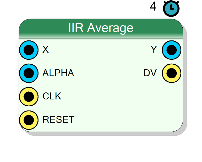
Pin Description
Properties
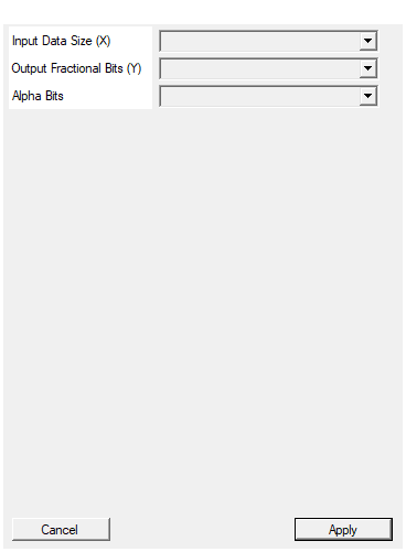
Bit width of input data X (8-24 bits)
Bit width of input data X. Range: 8-24 bits. Determines input precision and dynamic range.Default: 16
Options: 8 9 10 11 12 13 14 15 16 17 18 19 20 21 22 23 24
Number of fractional bits for output Y (0, 8, or 16)
Number of fractional bits in output Y:
- X.0: No fractional bits (output same size as input)
- X.8: 8 fractional bits added
- X.16: 16 fractional bits added More fractional bits improve precision for small alpha values.
Default: X.0
Options: X.0 X.8 X.16
Bit width of alpha coefficient (16, 24, or 32 bits)
Bit width of alpha coefficient:
- 16 bits: alpha resolution of 1/65536
- 24 bits: alpha resolution of 1/16777216
- 32 bits: alpha resolution of 1/4294967296 Higher resolution allows finer control of filter time constant.
Default: 16
Options: 16 24 32
Functional description
The IIR average implements a single-pole low-pass filter:
$$ y[n] = (1 - \alpha) \cdot y[n-1] + \alpha \cdot x[n] $$
where:
x[n]->X(input signal)y[n]->Y(filtered output)alpha->ALPHA(filter coefficient, 0 < alpha <= 1)
Transfer function
In the z-domain, the transfer function is:
$$ H(z) = \frac{\alpha}{1 - (1-\alpha) z^{-1}} $$
This corresponds to a first-order low-pass filter with:
- DC gain: 1 (unity)
- Pole at: $z = 1 - \alpha$
- Time constant: $\tau \approx 1/\alpha$ samples
Alpha coefficient
The ALPHA input is a fixed-point unsigned value representing a number
between 0 and 1:
| Alpha (decimal) | Effect | Equivalent samples |
|---|---|---|
| 1.0 | No filtering (y = x) | 1 |
| 0.5 | Fast response, moderate smoothing | 2 |
| 0.1 | Medium smoothing | 10 |
| 0.01 | Strong smoothing, slow response | 100 |
| 0.001 | Very strong smoothing | 1000 |
The alpha value is encoded as an unsigned integer where the full scale represents 1.0:
- 16-bit alpha: alpha = value / 65536
- 24-bit alpha: alpha = value / 16777216
- 32-bit alpha: alpha = value / 4294967296
Output precision
The output Y can have additional fractional bits for increased precision:
| Setting | Output bits | Description |
|---|---|---|
| X.0 | Same as X | Integer output only |
| X.8 | X bits + 8 fract | 8 fractional bits |
| X.16 | X bits + 16 fract | 16 fractional bits |
Additional fractional bits reduce quantization noise in the filter accumulator, important for small alpha values.
Internal accumulator
The accumulator size is automatically calculated to prevent overflow:
- Accumulator bits = X_DATA_BITS + Y_FRACT_BITS + ALPHA_BITS
This ensures full precision for all intermediate calculations.
Latency
Fixed latency of 4 clock cycles (HLS pipeline).
Typical use cases
- Exponential smoothing of sensor data
- Low-pass filtering with minimal resources
- Baseline tracking in spectroscopy
- DC offset estimation
- Signal envelope detection