
Mean Filter
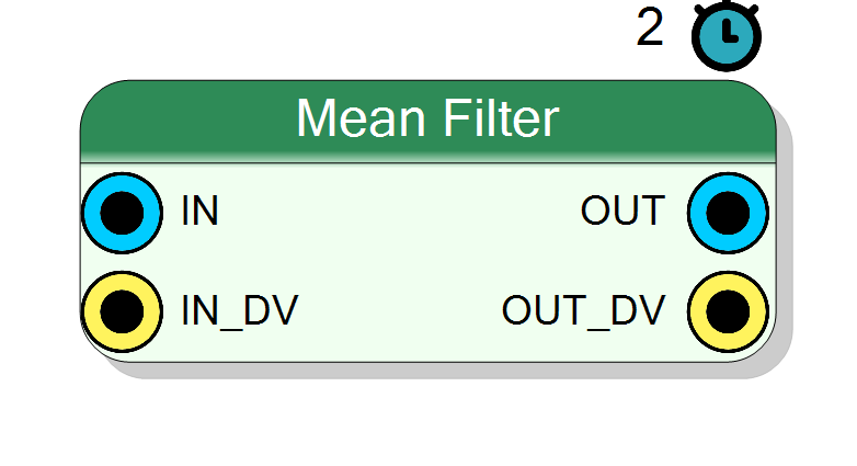
Sliding window arithmetic mean (moving average) in fixed point, with any window length from 2 to 64. Input and output have independently selectable integer bits, fractional bits and sign. Implemented as a running sum, so the cost does not grow with the window. Companion of the Median Filter, with the same pins and the same properties.
Introduction
The block outputs the arithmetic mean of the last WindowSize samples,
$$ \mathrm{OUT}(n) = \frac{1}{W}\sum_{k=0}^{W-1} x(n-k) $$
Mean or median?
This block and the Median Filter are drop-in alternatives – same pins, same properties – but they behave in opposite ways, and picking the wrong one is the usual reason a filter “does not work”:
| Mean Filter | Median Filter | |
|---|---|---|
| Gaussian / thermal noise | reduces it by $\sqrt{W}$ | barely helps |
| one huge outlier | spreads it over $W$ samples | discards it completely |
| step edge | smears it into a ramp | reproduces it as a step |
| narrow genuine pulse | attenuates it | removes it entirely |
| behaviour | linear, has a frequency response | non linear, has none |
In short: use the mean against random noise, the median against impulsive noise. A common arrangement is a short median first to kill the spikes, then a mean to reduce the residual random noise.
From the bottom: the raw input, this filter, and the Median Filter on the same signal. Both clean the baseline. The mean, being linear, also attenuates and widens the pulse – the peak comes out lower and later. The median leaves the edge intact. Use the mean when you want the smoothest baseline, the median when the shape of a transient matters.
Frequency response
Being linear, this filter does have a transfer function – the familiar sinc shape
$$ |H(f)| = \left| \frac{\sin(\pi f W / f_s)}{W \sin(\pi f / f_s)} \right| $$
with zeros at every multiple of $f_s / W$. That is worth knowing for two reasons: the stop band rejection is poor (the first sidelobe is only about 13 dB down), and the zeros can be placed deliberately – choosing $W = f_s / f_{disturb}$ nulls a known interfering tone exactly.
Pin Description
Properties
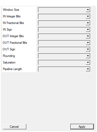
Number of samples averaged (2 to 64). The cost is one running sum regardless of the window length; powers of two divide with a plain shift and are exact.
Number of samples averaged, from 2 to 64.
Noise is reduced by $\sqrt{W}$ and the group delay is $(W-1)/2$ samples, so the window trades noise against response time. Powers of two divide with a plain shift and are bit exact; other lengths use a constant reciprocal accurate to well under one LSB. The arithmetic cost is the same either way.
Default: 8
Options: 2 3 4 5 6 7 8 9 10 11 12 13 14 15 16 17 18 19 20 21 22 23 24 25 26 27 28 29 30 31 32 33 34 35 36 37 38 39 40 41 42 43 44 45 46 47 48 49 50 51 52 53 54 55 56 57 58 59 60 61 62 63 64
Number of INTEGER bits of the input (the sign, when present, uses one of them).
Number of INTEGER bits of the input (1 to 64). When the input is SIGNED, one of these bits carries the sign.Default: 16
Options: 1 2 3 4 5 6 7 8 9 10 11 12 13 14 15 16 17 18 19 20 21 22 23 24 25 26 27 28 29 30 31 32 33 34 35 36 37 38 39 40 41 42 43 44 45 46 47 48 49 50 51 52 53 54 55 56 57 58 59 60 61 62 63 64
Number of FRACTIONAL bits of the input, i.e. the bits to the right of the binary point. Total input width = integer + fractional bits.
Number of FRACTIONAL bits of the input (0 to 64), i.e. the bits to the right of the binary point. Total input width = integer + fractional bits.Default: 0
Options: 0 1 2 3 4 5 6 7 8 9 10 11 12 13 14 15 16 17 18 19 20 21 22 23 24 25 26 27 28 29 30 31 32 33 34 35 36 37 38 39 40 41 42 43 44 45 46 47 48 49 50 51 52 53 54 55 56 57 58 59 60 61 62 63 64
Select whether the input is signed (two’s complement) or unsigned.
Arithmetic type of the input:
- SIGNED – two’s complement
- UNSIGNED – non negative only
Default: SIGNED
Options: UNSIGNED SIGNED
Number of INTEGER bits of the output.
Number of INTEGER bits of the output (1 to 64). An average never exceeds the range of its inputs, so the input integer width is always enough.Default: 16
Options: 1 2 3 4 5 6 7 8 9 10 11 12 13 14 15 16 17 18 19 20 21 22 23 24 25 26 27 28 29 30 31 32 33 34 35 36 37 38 39 40 41 42 43 44 45 46 47 48 49 50 51 52 53 54 55 56 57 58 59 60 61 62 63 64
Number of FRACTIONAL bits of the output. Set it equal to the input to keep the result exact; use more bits only if you widen the format elsewhere.
Number of FRACTIONAL bits of the output (0 to 64). Averaging produces resolution below the input LSB: adding two or three fractional bits here is what lets you keep it instead of rounding it away.Default: 0
Options: 0 1 2 3 4 5 6 7 8 9 10 11 12 13 14 15 16 17 18 19 20 21 22 23 24 25 26 27 28 29 30 31 32 33 34 35 36 37 38 39 40 41 42 43 44 45 46 47 48 49 50 51 52 53 54 55 56 57 58 59 60 61 62 63 64
Select whether the output is signed or unsigned.
Arithmetic type of the output, SIGNED or UNSIGNED.Default: SIGNED
Options: UNSIGNED SIGNED
ROUND: round to nearest when the output has fewer fractional bits than the input. TRUNCATE: drop them (cheaper, adds a negative bias).
- ROUND – round to nearest when fractional bits have to be discarded
- TRUNCATE – discard them (cheaper, introduces a negative bias that a long averaging chain will accumulate)
Default: ROUND
Options: TRUNCATE ROUND
YES: clip to the largest representable output value. NO: wrap around.
- YES – clip to the largest representable output value (symmetric, min = -max)
- NO – wrap around modulo the output width
Default: YES
Options: NO YES
Number of output register stages, i.e. extra latency in clock cycles. 0 takes the result straight out of the combinational logic.
Number of output register stages (0 to 8). Total latency is this value PLUS ONE, because the sliding window register is itself a clock. This is separate from the filter’s inherent $(W-1)/2$ sample group delay.Default: 1
Options: 0 1 2 3 4 5 6 7 8
Functional description
A shift register holds the last WindowSize samples and a running sum is maintained incrementally: on every valid sample the new value is added and the one leaving the window is subtracted. The sum is then divided by the window length.
The window advances only when IN_DV is high, so the filter also works on gated or
decimated streams.
Cost
Because the sum is maintained incrementally, the arithmetic cost is two adders regardless of the window length – a window of 64 costs the same as a window of 4. Only the shift register grows. No DSP slice is used when the window is a power of two.
The division by the window length is exact for every window, not only for the powers of two. The length is split as $W = 2^k \cdot P$ with $P$ odd; the $2^k$ is folded into the shift the output requantisation performs anyway, and the small odd factor $P$ (1 to 63) goes through a digit recurrence whose remainder is only 7 bits wide – a few LUTs per bit of the sum, no DSP and no reciprocal:
- powers of two (2, 4, 8, 16, 32, 64) – $P = 1$: the division disappears entirely into the requantisation shift and costs nothing
- any other length – a handful of LUTs, and the result is still the exactly rounded mean, not an approximation
Startup and reset
Reset clears both the window and the running sum. The first $W-1$ outputs after a reset therefore average a window that is still partly zero, and the output ramps up to the true average over the first $W$ samples. This is the same convention as a FIR filter starting from a cleared delay line.
Fixed-point format
Input and output carry their own Q format. A value with $N_{int}$ integer bits and $N_{frac}$ fractional bits occupies $N_{int} + N_{frac}$ bits and represents
$$ \text{value} = \frac{\text{raw integer}}{2^{N_{frac}}} $$
The internal sum is kept wide enough to hold $W$ full scale samples without overflow, so no headroom has to be reserved in the input format. Averaging never increases the magnitude of the signal, so an output format equal to the input one is always sufficient; giving the output a few extra fractional bits is the way to keep the resolution that the averaging actually buys you.
Latency
Total pipeline latency is PipelineLength + 1 clock cycles: the sliding window is itself
a register, and PipelineLength adds that many further output stages on top of it.
OUT_DV is delayed by the same amount, so the flag always travels with its sample – which
matters when IN_DV is gated rather than tied high.
This is separate from the filter’s own group delay of $(W-1)/2$ samples, inherent to any moving average.
Implementation
The block is generated with Vitis HLS from a shared parametric core
(Resources/Code/window_filter.cpp), which also serves the Median Filter: one source,
one requantiser, two reductions selected at synthesis time – so the two blocks cannot
drift apart on rounding, saturation or latency. Every property takes part in the IP
identity, so two placements with different settings get their own core and never
interfere. A Vitis HLS installation (or a remote build) is therefore required to compile
a design containing this block.
Relationship with Noise Filt. Moving Avg
This plugin already contains Noise Filt. Moving Avg, an older HLS implementation of the same operation restricted to windows of 4, 8, 16 or 32, with a fixed latency and no IN_DV gating. Mean Filter accepts any window from 2 to 64, works on gated streams, and exposes exactly the same properties as the Median Filter so the two can be swapped without rewiring. Either is fine for a plain moving average; prefer this one when you want to pair or swap it with the median.
Typical use cases
- Reducing random noise on a slowly varying signal
- Smoothing a baseline or a rate measurement
- Nulling a known interfering tone by placing a sinc zero on it
- Second stage after a Median Filter, to clean the residual random noise