
Rolling Variance
Real-time calculation of Mean, Variance and Sigma (standard deviation) over a configurable rolling window. Uses Welford-style incremental algorithm for efficient FPGA implementation.
Introduction
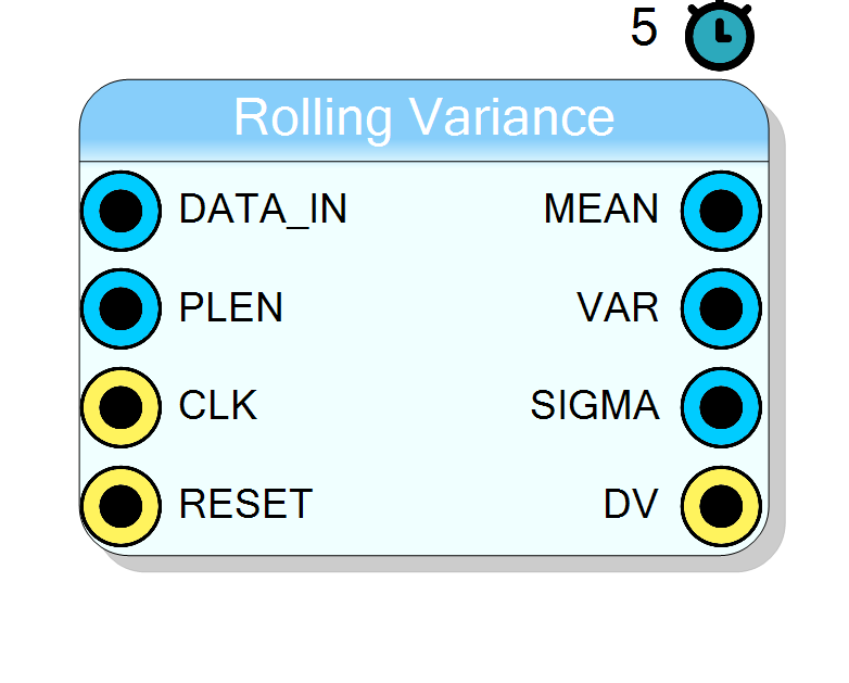
The Rolling Variance block calculates the Mean, Variance, and Sigma (standard deviation) in real time. Each sample provided to the DATA_IN input will update (after a pipeline delay of 5 clock cycles) the three output values.
Pin Description
Data Valid output.
- High (1): Mean, Variance, and Sigma outputs contain valid data
- Low (0): Outputs are invalid (during preroll or after PLEN change) Remains low for 2x Memory Size samples after reset or PLEN change.
Properties
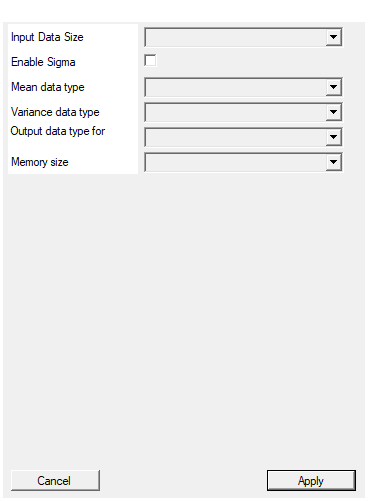
Number of bit of the input vector
Input data size in bits. Available values: 8, 16, 24, 32, default 16.Default: 16
Options: 8 16 24 32
Instantiate the square root module inside the core to calculate in realtime the sigma
Enable Sigma (standard deviation) calculation. When enabled, instantiates a square root module inside the core. Warning: Significantly increases FPGA resource usage. Default: Disabled.Default: False
Select data output type for mean
Output data type for Mean. Available values: fixed 32.32, fixed 32.16, fixed 32.8, fixed 24.8, fixed 16.16, int 16, int 32, int 64, fixed 56.8, fixed 48.16. Default: fixed 24.8.Default: fixed 24.8
Options: fixed 32.32 fixed 32.16 fixed 32.8 fixed 24.8 fixed 16.16 int 16 int 32 int 64 fixed 56.8 fixed 48.16
Select data output type for variance
Output data type for Variance. Available values: fixed 32.32, fixed 32.16, fixed 32.8, fixed 24.8, fixed 16.16, int 16, int 32, int 64, fixed 56.8, fixed 48.16. Default: fixed 24.8.Default: fixed 24.8
Options: fixed 32.32 fixed 32.16 fixed 32.8 fixed 24.8 fixed 16.16 int 16 int 32 int 64 fixed 56.8 fixed 48.16
Select data output type for sigma
Output data type for Sigma (standard deviation). Only used when “Enable Sigma” is checked. Available values: fixed 32.32, fixed 32.16, fixed 32.8, fixed 24.8, fixed 16.16, int 16, int 32, int 64, fixed 56.8, fixed 48.16. Default: fixed 16.16.Default: fixed 16.16
Options: fixed 32.32 fixed 32.16 fixed 32.8 fixed 24.8 fixed 16.16 int 16 int 32 int 64 fixed 56.8 fixed 48.16
Maximun number of samples in the rolling window
Maximum number of samples in the rolling window buffer. Determines the maximum valid PLEN value. Available values: 16, 32, 64, 128, 256, 512, 1024, 2048, 4096, 8192, 16384, 32768, 65536. Default: 1024.Default: 1024
Options: 16 32 64 128 256 512 1024 2048 4096 8192 16384 32768 65536
Usage
Mathematical Foundation
The variance is calculated using two running accumulators: one for the sum of values ($\sum x$) and another for the sum of squares ($\sum x^2$). This enables efficient incremental computation without storing all samples explicitly.
Variance Formula
The variance over N samples is computed as:
$$ \sigma^2 = \frac{\sum x^2}{N} - \left(\frac{\sum x}{N}\right)^2 $$
This is equivalent to the standard variance formula:
$$ \sigma^2 = \frac{1}{N}\sum_{i=1}^{N}(x_i - \bar{x})^2 $$
where $\bar{x}$ is the mean:
$$ \bar{x} = \frac{\sum x}{N} $$
The standard deviation (sigma) is simply the square root of the variance:
$$ \sigma = \sqrt{\sigma^2} $$
Rolling Window Algorithm
To achieve the rolling (sliding window) effect, incoming samples are stored in a circular buffer. The algorithm maintains two accumulators that are updated incrementally:
-
For each new sample $x_{new}$:
- Add $x_{new}$ to
sum - Add $x_{new}^2$ to
sum2
- Add $x_{new}$ to
-
For the oldest sample $x_{old}$ (N samples behind):
- Subtract $x_{old}$ from
sum - Subtract $x_{old}^2$ from
sum2
- Subtract $x_{old}$ from
This ensures that variance is always computed over the last N samples, providing the desired rolling window effect with O(1) complexity per sample.
Window Size Encoding (PLEN)
The window size N is encoded as a power of 2, specified by the PLEN input. This encoding allows efficient division using bit-shift operations instead of actual division.
| PLEN | Window Size (N) | Formula |
|---|---|---|
| 0 | INVALID | - |
| 1 | INVALID | - |
| 2 | INVALID | - |
| 3 | 8 | $2^3$ |
| 4 | 16 | $2^4$ |
| 5 | 32 | $2^5$ |
| 6 | 64 | $2^6$ |
| 7 | 128 | $2^7$ |
| 8 | 256 | $2^8$ |
| 9 | 512 | $2^9$ |
| 10 | 1024 | $2^{10}$ |
| 11 | 2048 | $2^{11}$ |
| 12 | 4096 | $2^{12}$ |
| 13 | 8192 | $2^{13}$ |
| 14 | 16384 | $2^{14}$ |
| 15 | 32768 | $2^{15}$ |
| 16 | 65536 | $2^{16}$ |
Important: The “Memory Size” property must be greater than or equal to the selected window size. For example, with Memory Size = 1024, valid PLEN values are 3 to 10.
Data Valid Signal (DV)
The DV output indicates when the Mean, Variance, and Sigma outputs contain valid data. When PLEN is changed (or at startup), DV is held low for at least 2 times the buffer size specified in the “Memory Size” property. This preroll period ensures the accumulators are properly initialized.
Fixed-Point Output Formats
Output data formats use fixed-point representation for fractional precision. The format notation fixed X.Y means:
- X bits: Integer part (including sign)
- Y bits: Fractional part
- Total bus width: X + Y bits
Example: fixed 24.8 = 24-bit integer + 8-bit fractional = 32-bit total
Resources & Timing
-
Latency: 5 clock cycles
-
Throughput: 1 sample per clock cycle (II=1)
HLS-based implementation. Resource usage varies with configuration.