
Tunable IIR - II Order
Second-order IIR filter with user-programmable coefficients. Allows runtime coefficient updates for adaptive filtering applications.
Introduction
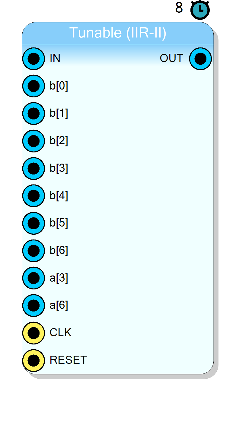
The Tunable IIR - II Order block implements a second-order IIR filter (biquad) with user-programmable coefficients operating in real time on FPGA. Unlike fixed-coefficient filters (Butterworth, Chebyshev, etc.), this block allows the user to provide custom filter coefficients that can be changed at runtime.
This component is ideal for adaptive filtering applications where the filter response must be adjusted dynamically based on system conditions.
Pin Description
Properties
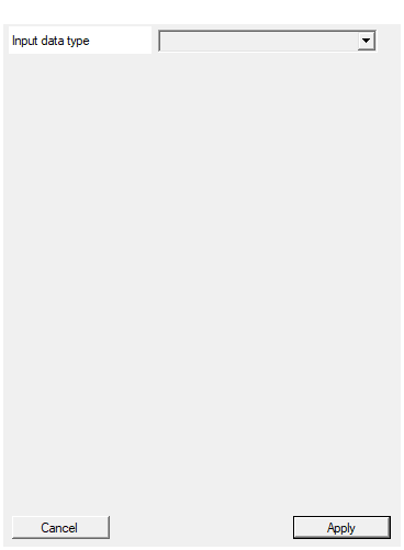
Select input data type
Input data format selection. Available values: Unsigned 16 bit, Signed 17 bit, default Unsigned 16 bit.Default: UINT16
Options: UINT16 INT17
Usage
Second-Order IIR Filter Theory
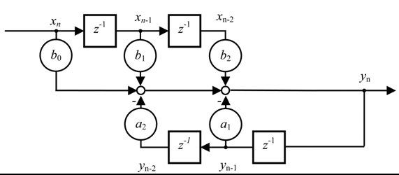
A standard second-order IIR filter (biquad) is described by the difference equation:
$$ y[n] = b_0 x[n] + b_1 x[n-1] + b_2 x[n-2] - a_1 y[n-1] - a_2 y[n-2] $$
In Z-domain, the transfer function is:
$$ H(z) = \frac{b_0 + b_1 z^{-1} + b_2 z^{-2}}{1 + a_1 z^{-1} + a_2 z^{-2}} $$
The recursive dependencies on $y[n-1]$ and $y[n-2]$ create feedback loops that limit the maximum clock rate on FPGA implementations.
Scattered Lookahead Transformation
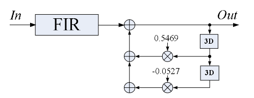
To enable high-speed FPGA operation, the filter uses the Scattered Lookahead technique. This transforms the original filter into an equivalent form where feedback dependencies span 3 and 6 samples instead of 1 and 2.
Reference: A universal look-ahead algorithm for pipelining IIR filters
Mathematical Derivation
Starting from the original second-order filter in matrix form. Define the state vector and coefficient matrices:
Original filter: $y[n] = b_0 x[n] + b_1 x[n-1] + b_2 x[n-2] - a_1 y[n-1] - a_2 y[n-2]$
We construct the A matrix (lower triangular Toeplitz) representing the denominator polynomial convolution:
$$ \mathbf{A} = \begin{bmatrix} a_0 & 0 & 0 & 0 & 0 \ a_1 & a_0 & 0 & 0 & 0 \ a_2 & a_1 & a_0 & 0 & 0 \ 0 & 0 & a_2 & a_1 & a_0 \ 0 & 0 & 0 & a_2 & a_1 \end{bmatrix} $$
where $a_0 = 1$ (normalized filter).
Step 1: Compute the Inverse
Calculate $\mathbf{A}^{-1}$, then extract the first column:
$$ \mathbf{D} = \mathbf{A}^{-1} \cdot \begin{bmatrix} 1 \ 0 \ 0 \ 0 \ 0 \end{bmatrix} $$
The vector $\mathbf{D} = [d_0, d_1, d_2, d_3, d_4]^T$ contains the coefficients for the numerator transformation.
Step 2: Compute Feedback Coefficients
Define the R matrix for extracting feedback terms:
$$ \mathbf{R} = \begin{bmatrix} 0 & a_2 & a_1 & a_0 & 0 \ 0 & 0 & 0 & 0 & a_2 \end{bmatrix} $$
Compute:
$$ \mathbf{Q} = \mathbf{R} \cdot \mathbf{D} $$
The transformed feedback coefficients are:
$$ a’_3 = Q_0, \quad a’_6 = Q_1 $$
Step 3: Transform Numerator
The transformed numerator is obtained by convolving $\mathbf{D}$ with the original numerator:
$$ b’[n] = \mathbf{D} * b[n] = \text{conv}([d_0, d_1, d_2, d_3, d_4], [b_0, b_1, b_2]) $$
This produces 7 coefficients: $b’_0, b’_1, b’_2, b’_3, b’_4, b’_5, b’_6$
Transformed Filter Equation
The FPGA implements:
$$ y[j] = \sum_{k=0}^{6} b’_k x[j-k] - a’_3 y[j-3] - a’_6 y[j-6] $$
This form allows:
- 3 clock cycles between first feedback ($y[j-3]$)
- 6 clock cycles between second feedback ($y[j-6]$)
Stability Analysis
The stability of the transformed filter depends on the pole locations of the original filter.
Original Filter Stability Conditions
For a second-order filter with denominator $1 + a_1 z^{-1} + a_2 z^{-2}$, the poles are:
$$ p_{1,2} = \frac{-a_1 \pm \sqrt{a_1^2 - 4a_2}}{2} $$
The filter is stable if and only if both poles lie inside the unit circle. This is equivalent to the Jury stability criterion:
$$ |a_2| < 1 $$ $$ |a_1| < 1 + a_2 $$
Transformed Filter Stability
The scattered lookahead transformation preserves the poles of the original filter. The transformation is mathematically equivalent - it only restructures the computation, not the transfer function.
Therefore:
- If the original filter is stable, the transformed filter is stable
- If the original filter is unstable, the transformed filter is also unstable
Practical verification: After transformation, verify:
- Frequency response magnitude matches the original
- Pole locations (roots of denominator) remain inside unit circle
Fixed-Point Coefficient Format
The FPGA implementation uses 32-bit signed fixed-point coefficients with 30 fractional bits (Q2.30 format):
$$ \text{coefficient}{fixed} = \text{round}(\text{coefficient}{float} \times 2^{30}) $$
This provides:
- Range: approximately $\pm 2$
- Precision: approximately $9.3 \times 10^{-10}$
Python Reference Implementation
The following Python code calculates the transformed coefficients for any second-order IIR filter:
python
import numpy as np
from scipy import signal
def scattered_lookahead_transform(a):
"""
Apply scattered lookahead transformation to second-order IIR denominator.
Parameters:
a: array [a0, a1, a2] where a0=1 (normalized denominator coefficients)
Returns:
bn: numerator transformation coefficients [d0, d1, d2, d3, d4]
an: transformed denominator [1, a'3, a'6]
"""
# Construct the A matrix (lower triangular Toeplitz)
A = np.array([[a[0], 0, 0, 0, 0 ],
[a[1], a[0], 0, 0, 0 ],
[a[2], a[1], a[0], 0, 0 ],
[0, 0, a[2], a[1], a[0]],
[0, 0, 0, a[2], a[1]]])
# Compute inverse and extract first column
A_inv = np.linalg.inv(A)
D = A_inv @ np.array([1, 0, 0, 0, 0])
# R matrix for feedback coefficient extraction
R = np.array([[0, a[2], a[1], a[0], 0 ],
[0, 0, 0, 0, a[2]]])
# Compute transformed feedback coefficients
Qw = R @ D
an = [1, Qw[0], Qw[1]] # Transformed denominator
bn = D # Numerator transformation coefficients
return bn, an
# Example: Design a second-order Butterworth low-pass filter
N = 2 # Order of filter
fs = 250e6 # Sampling frequency (Hz)
fc = 10e6 # Cutoff frequency (Hz)
Wn = fc / (fs / 2) # Normalized frequency
# Get original filter coefficients
b_z, a_z = signal.butter(N, Wn, btype='low')
print("Original coefficients:")
print(f" b = {b_z}")
print(f" a = {a_z}")
# Apply scattered lookahead transformation
bn, an = scattered_lookahead_transform(a_z)
# Compute final numerator by convolution
bq = np.convolve(bn, b_z)
print("\nTransformed coefficients (scattered lookahead):")
print(f" b' = {bq}")
print(f" a' = {an}")
# Verify frequency response equivalence
w_orig, h_orig = signal.freqz(b_z, a_z, worN=1024)
w_trans, h_trans = signal.freqz(bq, an, worN=1024)
print("\nFrequency response verification:")
print(f" Max magnitude difference: {np.max(np.abs(np.abs(h_orig) - np.abs(h_trans))):.2e}")
# Stability analysis
print("\nStability analysis:")
poles_orig = np.roots(a_z)
poles_trans = np.roots(an)
print(f" Original poles: {poles_orig}")
print(f" |poles| = {np.abs(poles_orig)}")
print(f" Original filter: {'STABLE' if np.all(np.abs(poles_orig) < 1) else 'UNSTABLE'}")
# Convert to fixed-point (Q2.30 format)
SCALE = 1 << 30
b_fixed = [int(round(c * SCALE)) for c in bq]
a_fixed = [int(round(c * SCALE)) for c in an]
print("\nFixed-point coefficients (Q2.30):")
print(" Numerator (b coefficients):")
for i, c in enumerate(b_fixed):
print(f" b[{i}] = {c}")
print(" Denominator (a coefficients):")
print(f" a[3] = {a_fixed[1]}")
print(f" a[6] = {a_fixed[2]}")
Coefficient Summary Table
| Pin | Coefficient | Description |
|---|---|---|
| b[0] | $b’_0$ | First feedforward tap |
| b[1] | $b’_1$ | Second feedforward tap |
| b[2] | $b’_2$ | Third feedforward tap |
| b[3] | $b’_3$ | Fourth feedforward tap |
| b[4] | $b’_4$ | Fifth feedforward tap |
| b[5] | $b’_5$ | Sixth feedforward tap |
| b[6] | $b’_6$ | Seventh feedforward tap |
| a[3] | $a’_3$ | First feedback (3-sample delay) |
| a[6] | $a’_6$ | Second feedback (6-sample delay) |
Typical Applications
- Adaptive filtering with runtime coefficient updates
- Custom filter responses not available in standard blocks
- Parametric equalizers with adjustable frequency/Q
- System identification and modeling
- Real-time filter tuning based on environmental conditions
- Research and prototyping of custom filter designs
- Notch/peak filters with adjustable center frequency
Resources & Timing
- Latency: 8 clock cycles