
FFT
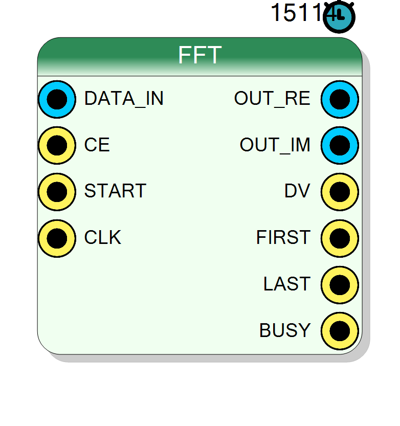
Fast Fourier Transform (FFT) engine built on top of the Xilinx FFT IP core. Supports configurable transform lengths from 128 to 16384 points, multiple algorithm architectures (Pipelined, Radix-4, Radix-2, Radix-2-Lite), 16-bit input and 32-bit complex output (real and imaginary parts).
Introduction
The block computes the Fast Fourier Transform of an input time-domain sequence. The transform converts time-domain samples into frequency-domain complex coefficients.
On every rising edge of CLK, when CE = 1 and after a START pulse
initiates the transform, the core accepts samples on DATA_IN and produces
complex frequency-domain output as separate real (OUT_RE) and imaginary
(OUT_IM) parts.
$$ X[k] = \sum_{n=0}^{N-1} x[n] \cdot e^{-j2\pi kn/N}, \quad k = 0, 1, \ldots, N-1 $$
where $N$ is the Length property (transform size).
The internal datapath is implemented with the Xilinx FFT IP core. Different Algorithm options trade off throughput, latency, and resource usage.
Pin Description
START.
CE = 0, the FFT core pauses operation and does not accept
new input samples or produce outputs.
DATA_IN with CE = 1 after START.
DV_OUT = 1. Outputs are produced in natural order
(bin 0, 1, 2, …, $N-1$).
DV_OUT = 1. For real-only input, expect $X[0]$ and
$X[N/2]$ to have zero imaginary parts.
OUT_RE and OUT_IM contain valid frequency-domain
samples. Pulses high for $N$ consecutive cycles (one per output bin).
BUSY = 1.
Properties
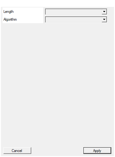
Select length of the FFT transform
FFT transform length $N$ (number of points). Allowed values: 128, 256, 512, 1024, 2048, 4096, 8192, 16384. Larger transforms provide finer frequency resolution: $$ \Delta f = \frac{f_s}{N} $$ where $f_s$ is the sampling rate. Changing this value re-configures the underlying FFT IP core.Default: 4096
Options: 128 256 512 1024 2048 4096 8192 16384
Select algorithm used to calculate FFT. Pipelined is faster but require much more resources than others algorithms.
Selects the FFT algorithm architecture:
- Pipelined: Highest throughput, highest resource usage. Continuous streaming capable.
- Radix-4: Balanced performance and resources. Burst I/O.
- Radix-2: Lower resources, moderate latency. Burst I/O.
- Radix-2-Lite: Minimal resources, longest latency. Best for area-constrained designs.
The choice affects latency, throughput, and FPGA resource consumption (DSP slices, block RAM, logic).
Default: Radix-4
Options: Pipelined Radix-4 Radix-2 Radix-2-Lite
Functional description
The component realizes the Discrete Fourier Transform (DFT):
$$ X[k] = \sum_{n=0}^{N-1} x[n] \cdot e^{-j2\pi kn/N} $$
where:
- $x[n]$ → time-domain input samples on
DATA_IN - $X[k]$ → frequency-domain output as
OUT_RE[k] + j \cdot OUT_IM[k] - $N$ → transform length (128, 256, …, 16384)
Input and Output
Input: 16-bit signed fixed-point samples representing real time-domain data.
Output: 32-bit signed fixed-point complex numbers:
OUT_RE: Real part of $X[k]$OUT_IM: Imaginary part of $X[k]$
Control signals
START: Pulse high to begin a new FFT transform. AfterSTART, feed exactly $N$ samples onDATA_INwithCE = 1.CE: Clock enable; when low, the core pauses.DV_OUT: Data valid output; high when valid frequency-domain samples are available onOUT_REandOUT_IM.FIRST: Pulses high on the first output sample ($k=0$) of a transform.LAST: Pulses high on the last output sample ($k=N-1$) of a transform.BUSY: High while the FFT engine is processing a transform.
Algorithm architectures
The Xilinx FFT core supports multiple architectures:
| Algorithm | Throughput | Resource usage | Latency (approx.) |
|---|---|---|---|
| Pipelined | Very high | Very high | $3N + 137$ |
| Radix-4 | Medium | Medium | $3.79N - 401$ |
| Radix-2 | Low | Low | $9.09N - 2436$ |
| Radix-2-Lite | Very low | Very low | $16.15N - 5280$ |
where $N$ is the transform length.
- Pipelined: Continuous streaming; new transform can start every $N$ cycles.
- Radix-4/Radix-2: Burst I/O; lower resource usage but longer processing time.
- Radix-2-Lite: Minimal resources; best for resource-constrained designs.
Mathematical background
The FFT is an efficient algorithm to compute the DFT with complexity $O(N \log_2 N)$ instead of $O(N^2)$ for direct computation.
The output $X[k]$ represents the amplitude and phase of the frequency component at bin $k$:
$$ f_k = k \cdot \frac{f_s}{N} $$
where $f_s$ is the sampling frequency.
Timing and latency
Latency varies by algorithm and transform length:
| Length | Pipelined | Radix-4 | Radix-2 | Radix-2-Lite |
|---|---|---|---|---|
| 128 | 521 | 84 | -1272 | -3213 |
| 1024 | 3209 | 3477 | 6773 | 11277 |
| 4096 | 12425 | 15119 | 34780 | 60947 |
(Negative values in the table indicate formula extrapolation outside valid range.)
The component reports the calculated latency in the Latency property of
the symbol.
Typical use cases
- Spectrum analysis in SDR receivers
- OFDM modulation/demodulation (LTE, Wi-Fi, DVB-T)
- Vibration analysis in structural health monitoring
- Audio processing and equalization
- Radar and sonar signal processing
- Nuclear/particle physics (pulse shape analysis in frequency domain)
Waveform example
Simplified timing for an 8-point FFT (Radix-2):