
IIR Butterworth - II Order
Second-order Butterworth IIR filter with maximally flat passband response. Provides smooth transition between passband and stopband with no ripples.
Introduction
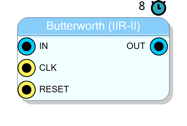
The IIR Butterworth - II Order block implements a second-order IIR (Infinite Impulse Response) filter operating in real time on FPGA. The component includes automatic filter coefficient calculation based on filter type (low/high pass) and cutoff frequency.
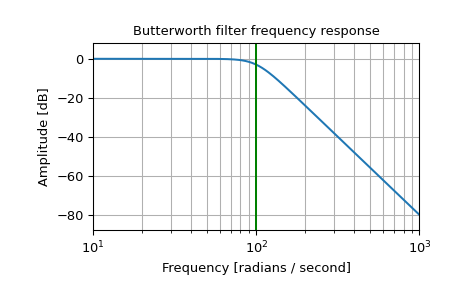
The Butterworth filter is widely used due to its maximally flat frequency response in the passband, meaning it does not have any ripples like Chebyshev or Elliptic filters.
Pin Description
Properties
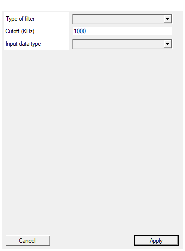
Select between low pass and high pass filter
Filter type selection. Available values: Low Pass, High Pass, default Low Pass.Default: Low Pass
Options: Low Pass High Pass
Set the filter pole/zero position according to the selected bandwidth in KHz
Cutoff frequency in kHz. Must be less than half the sampling frequency (Nyquist limit).Default: 1000
Select input data type
Input data format selection. Available values: Unsigned 16 bit, Signed 17 bit, default Unsigned 16 bit.Default: UINT16
Options: UINT16 INT17
Usage
Butterworth Filter Characteristics
The Butterworth filter’s design is based on the Butterworth polynomial, which defines its transfer function. Key characteristics include:
-
Maximally Flat Passband: The gain does not fluctuate and remains maximally flat, avoiding any distortion from ripples.
-
Monotonic Decrease: Both in passband and stopband, the filter’s response decreases monotonically without oscillations.
-
Pole Placement: The poles are placed on a circle in the z-plane and are evenly spaced, ensuring smooth transition characteristics.
Scattered Lookahead Implementation
To enable real-time FPGA operation at full clock rate, the filter uses the Scattered Lookahead technique. This transforms the recursive IIR structure to allow pipelined parallel processing:
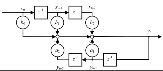
The standard IIR equation:
$$ y[n] = b_0 x[n] + b_1 x[n-1] + b_2 x[n-2] - a_1 y[n-1] - a_2 y[n-2] $$
Is transformed using scattered lookahead to:
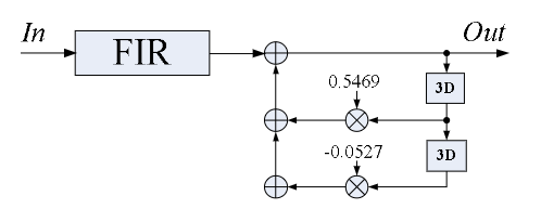
$$ y[j] = \sum_{k=0}^{6} b’_k x[j-k] - a’_3 y[j-3] - a’_6 y[j-6] $$
Reference: A universal look-ahead algorithm for pipelining IIR filters
Coefficient Calculation
SciCompiler automatically calculates the filter coefficients using the internal filter calculator tool. The following Python code provides a reference implementation for offline simulation:
python
import numpy as np
from scipy import signal
def scattered_lookahead_transform(a):
A = np.array([[a[0], 0, 0, 0, 0, ],
[a[1], a[0], 0, 0, 0, ],
[a[2], a[1], a[0], 0, 0, ],
[0, 0, a[2], a[1], a[0], ],
[0, 0, 0, a[2], a[1], ]])
A_inv = np.linalg.inv(A)
D = A_inv * [1, 0, 0, 0, 0]
D1 = D[:,0]
D = D[:,0].reshape(-1, 1)
R = np.array([[ 0, a[2], a[1], a[0], 0, ],
[0, 0, 0, 0, a[2]]])
Qw = np.dot(R, D)
an = [1, Qw[0][0], Qw[1][0]]
bn = D1
return bn, an
N = 2 # Order of the filter
fs = 250*1e6 # Sampling frequency
fc = 5*1e6 # Corner frequency
Wn = fc/(fs/2)
b_z, a_z = signal.butter(N, Wn, btype='low')
print("original", b_z, a_z)
bn, an = scattered_lookahead_transform(a_z)
bq = np.convolve(bn, b_z)
aq = an
print("scattered", bq, aq)
Typical Applications
- General-purpose signal filtering with smooth frequency response
- Anti-aliasing filters
- Audio signal processing
- Applications requiring uniform passband behavior
Resources & Timing
- Latency: 8 clock cycles