
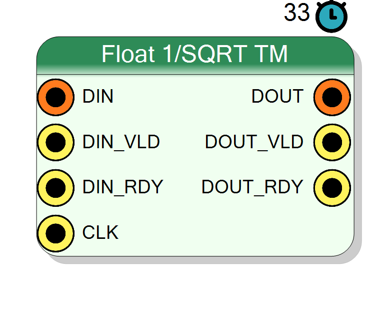
Float 1/SQRT TM
Time-multiplexed reciprocal square root operator for IEEE 754 floating-point numbers based on Xilinx Floating Point IP. Computes 1/sqrt(x) with single (32-bit) or double (64-bit) precision, configurable DSP usage, and multiple TM phases (1-32) for high-throughput parallel computation in signal normalization and graphics applications.
Introduction
This block computes the reciprocal square root (inverse square root) of IEEE 754 floating-point values using the Xilinx Floating Point IP core. The component supports Time Multiplexing (TM): multiple parallel computation units share the same clock cycle.
On every rising edge of CLK, if DIN_VLD = 1 and DOUT_RDY = 1:
$$ \mathrm{DOUT}(n) = \frac{1}{\sqrt{\mathrm{DIN}(n)}} $$
Pin Description
Properties
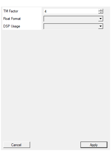
Time Multiplexing factor (number of phases)
Number of TM phases (1 – 32).Default: 4
Range: 1 – 32
Select between single precision 32 bit and double precision 64 bit
Single or Double precision.Default: Single
Options: Single Double
DSP Usage. Single precision: No [0], Full[9]. Double precision: No[0], Full[75]
No_UsageorFull_UsageSingle: 0/9 DSPs; Double: 0/75 DSPs
Default: Full_Usage
Options: No_Usage Full_Usage
Functional description
Wraps Xilinx Floating Point IP (operation type: Rec_Square_Root) with N parallel
instances for TM support.
Mathematical background
Reciprocal square root function:
$$ y = \frac{1}{\sqrt{x}} = x^{-1/2} $$
Properties:
- $\frac{1}{\sqrt{1}} = 1$
- $\frac{1}{\sqrt{x}} = \frac{\sqrt{x}}{x}$
- More efficient than computing sqrt then reciprocal separately
- Undefined for $x \leq 0$ (returns NaN for negative, Inf for zero)
Timing
Fixed latency of 33 clock cycles per phase.
| Property | Latency (cycles) |
|---|---|
| Reciprocal Sqrt | 33 |
DSP Usage
- Single precision: No [0], Full[9]
- Double precision: No[0], Full[75]
Typical use cases
- Fast vector normalization
- Graphics (lighting calculations)
- Machine learning (batch normalization)
- Fast Fourier Transform scaling
- Collision detection
- Quake III fast inverse square root replacement