
ALU - NOISE FILTER FIR
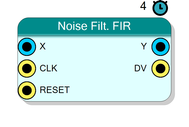
Advanced FIR low-pass noise filter with optimized coefficients generated via scipy.signal.firwin. Uses symmetric coefficients for linear phase response and resource optimization. Configurable order and cutoff frequency.
Introduction
The Noise Filter FIR block implements an advanced FIR low-pass filter:
$$ y[n] = \sum_{k=0}^{N-1} h[k] \cdot x[n-k] $$
where:
Nis the number of taps (5, 7, 9, 11, 13, or 15)h[k]are the filter coefficients generated by scipy.signal.firwin- Hamming window is used for optimal sidelobe suppression
This filter offers:
- Better frequency response than simple moving average
- Configurable cutoff frequency
- Linear phase (symmetric coefficients)
- Reduced ripple in passband and stopband
Pin Description
Properties
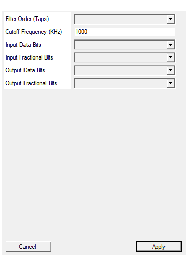
Number of FIR filter taps (5, 7, 9, 11, 13, or 15). Higher values give sharper cutoff but more latency.
Number of FIR filter taps (coefficients). Options: 5, 7, 9, 11, 13, or 15.
Trade-offs:
- 5 taps: Minimal resources, wide transition band
- 9 taps: Good balance of performance and resources
- 15 taps: Sharpest cutoff, most resources
For noise filtering, 7-11 taps is usually sufficient.
Default: 9
Options: 5 7 9 11 13 15
Low-pass filter cutoff frequency in KHz. Must be less than half the sampling frequency.
Low-pass filter cutoff frequency in KHz. Must be less than half the sampling frequency (Nyquist).
The cutoff is the -3dB point (half power).
Example: For 125 MHz sampling, max cutoff is 62.5 MHz (62500 KHz). Typical values: 1000-10000 KHz for noise filtering.
Default: 1000
Total bit width of input data (8-32 bits)
Total bit width of input data X. Range: 8-32 bits. Includes both integer and fractional parts.Default: 16
Options: 8 9 10 11 12 13 14 15 16 17 18 19 20 21 22 23 24 25 26 27 28 29 30 31 32
Number of fractional bits in input data (0-16)
Number of fractional bits in input data. Range: 0-16 bits. Integer bits = InDataBits - InFractBits.Default: 0
Options: 0 1 2 3 4 5 6 7 8 9 10 11 12 13 14 15 16
Total bit width of output data (8-64 bits)
Total bit width of output data Y. Range: 8-64 bits. Should be at least InDataBits for no precision loss.Default: 16
Options: 8 9 10 11 12 13 14 15 16 17 18 19 20 21 22 23 24 25 26 27 28 29 30 31 32 33 34 35 36 37 38 39 40 41 42 43 44 45 46 47 48 49 50 51 52 53 54 55 56 57 58 59 60 61 62 63 64
Number of fractional bits in output data (0-32)
Number of fractional bits in output data. Range: 0-32 bits. For best precision, match InFractBits.Default: 0
Options: 0 1 2 3 4 5 6 7 8 9 10 11 12 13 14 15 16 17 18 19 20 21 22 23 24 25 26 27 28 29 30 31 32
Functional description
The FIR filter computes the convolution of input samples with the impulse response:
$$ y[n] = h_0 \cdot x[n] + h_1 \cdot x[n-1] + \ldots + h_{N-1} \cdot x[n-N+1] $$
Coefficient generation
Coefficients are generated at compile time using Python’s scipy.signal.firwin with a Hamming window. This provides:
- Good sidelobe attenuation: ~-43 dB first sidelobe
- Smooth frequency response: Minimal ripple
- Linear phase: Symmetric coefficients preserve waveform shape
Symmetric coefficient optimization
Since coefficients are symmetric (h[k] = h[N-1-k]), the implementation exploits this to reduce multiplications:
$$ y[n] = \sum_{k=0}^{\lfloor N/2 \rfloor} h[k] \cdot (x[n-k] + x[n-N+1+k]) $$
For a 9-tap filter, this reduces multiplications from 9 to 5.
Transfer function
In the z-domain:
$$ H(z) = \sum_{k=0}^{N-1} h[k] \cdot z^{-k} $$
Comparison with Moving Average
| Feature | Moving Average | FIR (Hamming) |
|---|---|---|
| Passband ripple | High (sinc response) | Low |
| Stopband attenuation | -13 dB (first null) | -43 dB |
| Transition band | Wide | Sharper |
| Phase | Linear | Linear |
| Complexity | Simple (shift/add) | Multipliers |
Filter order selection
| Taps | Transition bandwidth | Stopband attenuation |
|---|---|---|
| 5 | ~0.4 * fs | -30 dB |
| 7 | ~0.3 * fs | -35 dB |
| 9 | ~0.25 * fs | -40 dB |
| 11 | ~0.2 * fs | -43 dB |
| 13 | ~0.17 * fs | -45 dB |
| 15 | ~0.15 * fs | -47 dB |
Higher order = sharper cutoff but more latency and resources.
Resource usage
- N/2 + 1 multipliers (symmetric optimization)
- N delay registers
- Adder tree for accumulation
Latency
Fixed latency of 4 clock cycles (HLS pipeline). The DV output goes high after N samples have been processed.
Typical use cases
- ADC noise reduction with precise cutoff
- Anti-aliasing filters
- Signal conditioning
- Decimation pre-filters
- Band-limiting for oversampled signals